How should sparse marine in situ measurements be compared to a continuous model: an example

(1)

Geosci. Model Dev., 6, 533–548, 2013 www.geosci-model-dev.net/6/533/2013/ doi:10.5194/gmd-6-533-2013

EGU Journal Logos (RGB)

Advances in

Geosciences

Open Access

Natural Hazards

and Earth System

Sciences

Open Access

Annales

Geophysicae

Open Access

Nonlinear Processes

in Geophysics

Open Access

Atmospheric

Chemistry

and Physics

Open Access

Atmospheric

Chemistry

and Physics

Open Access Discussions

Atmospheric

Measurement

Techniques

Open Access

Atmospheric

Measurement

Techniques

Biogeosciences

Open Access Open Access

Biogeosciences

Discussions

Climate

of the Past

Climate

of the Past

Discussions

Earth System

Dynamics

Earth System

Dynamics

Discussions

Geoscientific

Instrumentation

Methods and

Data Systems

Open Access

_{Geoscientific}

Instrumentation

Methods and

Data Systems

Geoscientific

Model Development

Geoscientific

Model Development

Discussions

Hydrology and

Earth System

Sciences

Open Access

Hydrology and

Earth System

Sciences

Ocean Science

Discussions

Solid Earth

Discussions

The Cryosphere

Discussions

Natural Hazards

and Earth System

Sciences

Open Access

Discussions

How should sparse marine in situ measurements be compared to

a continuous model: an example

L. de Mora, M. Butensch¨on, and J. I. Allen

Plymouth Marine Laboratory, Prospect Place, The Hoe, Plymouth, PL1 3DH, UK

Correspondence to: L. de Mora ([email protected])

Received: 18 July 2012 – Published in Geosci. Model Dev. Discuss.: 20 August 2012 Revised: 22 March 2013 – Accepted: 4 April 2013 – Published: 25 April 2013

Abstract. This work demonstrates an example of the

impor-tance of an adequate method to sub-sample model results when comparing with in situ measurements. A test of model skill was performed by employing a point-to-point method to compare a multi-decadal hindcast against a sparse, un-evenly distributed historic in situ dataset. The point-to-point method masked out all hindcast cells that did not have a cor-responding in situ measurement in order to match each in situ measurement against its most similar cell from the model. The application of the point-to-point method showed that the model was successful at reproducing the inter-annual vari-ability of the in situ datasets. Furthermore, this success was not immediately apparent when the measurements were ag-gregated to regional averages. Time series, data density and target diagrams were employed to illustrate the impact of switching from the regional average method to the point-to-point method. The comparison based on regional averages gave significantly different and sometimes contradicting re-sults that could lead to erroneous conclusions on the model performance. Furthermore, the point-to-point technique is a more correct method to exploit sparse uneven in situ data while compensating for the variability of its sampling. We therefore recommend that researchers take into account for the limitations of the in situ datasets and process the model to resemble the data as much as possible.

1 Introduction

Numerical models are now used extensively in earth, cli-mate and ocean sciences. Furthermore, numerical models are frequently used to inform policy decisions. Both pol-icy decision and fundamental science require models to have

demonstrable quality. However, the assessment of how well a model captures reality is an ongoing challenge of marine ecosystem model development.

As discussed in a meta-analysis (Arhonditsis and Brett, 2004), many models have been validated with qualita-tive methods exclusively. Qualitaqualita-tive methods are usually straightforward to interpret, allowing for a simple, fast, sub-jective judgement of whether the model appears to be repre-sentative of the measurements. Unfortunately, a model may seem to recreate emergent properties and well-known large-scale features of the ecosystem, yet struggle to reproduce the historic data of a hindcast, for instance Doney et al. (2009). For these reasons, it is crucial to validate models using a va-riety of objective statistical tests.

In marine ecosystem modelling, quantitative descriptions of models are often based on pattern statistics, and other uni-variate indices, for instance in Stow et al. (2009). Pattern statistics form the axes of the popular Taylor (Taylor, 2001) and target diagrams (Jolliff et al., 2009). These univariate in-dices generally require equal binning of (i.e. the same num-ber of) both model and measurement data, but the method-ology used to achieve equal binning can introduce sampling bias.

(2)

structure, it is extremely difficult to interpolate sparse ma-rine in situ measurements at depth into a three-dimensional grid. Typically, 3-D interpolation assumes that all axes have equal weight, but in the ocean, the vertical scale varies in dis-tances of metres and the horizontal scales in kilometres. It is not straightforward to choose whether a pixel should be more influenced by a deeper nearby point or by a distant point of similar depth.

Alternatively, the equal binning condition can be achieved by taking the mean of both the model and in situ data over a sufficiently large region, as in Lewis et al. (2006). When the data are three-dimensional marine in situ measurements, choosing an appropriate mean can be a challenge as the mean of an arbitrary set of marine in situ measurements in three di-mensions is unlikely to be a good indicator of the typical state of the system. Further sampling bias is introduced when the mean of measurements of a very small subset of the ocean is compared against the mean of a very large volume in the model. These problems are compounded when ad hoc sam-pling is further biased toward coastal sites that are both ac-cessible and convenient.

In this paper, a point-to-point method is outlined to val-idate a marine ecosystem model hindcast in using historic in situ measurements in the politically significant North Sea region. The point-to-point method does not introduce new uncertainties via interpolation and attempts to reduce the im-pact of sampling bias introduced via historic ad hoc sam-pling. While it may seem obvious to process the model ex-actly as the in situ data were produced, it seems to have rarely been done in marine biogeochemical modelling, or published with a lack of transparency. Furthermore, to the best of the authors’ knowledge, this is the first direct comparison of the matched against unmatched methodologies.

The model used in this study is the European Regional Seas Ecosystem Model (ERSEM) coupled with the Proud-man Oceanographic Laboratory Coastal-Ocean Modelling System (POLCOMS) as described in Sects. 2 and 3. The in situ data are the Conductivity, Temperature and Depth (CTD) sampler data and low-resolution bottle data in the North Sea from the International Council of the Sea (ICES) database, described in Sect. 4. A full description of the methodology of the point-to-point matching and the linear regression is in Sect. 5. The agreement of the in situ and model data, and a comparison of matched and unmatched methods are shown in Sect. 6.

2 Circulation model

The Proudman Oceanographic Laboratory Coastal-Ocean Modelling System (POLCOMS) hydrodynamic model (Holt et al., 2001) is a baroclinic three-dimensional model that in-cludes both the deep ocean and the continental shelf.

This study used POLCOMS-ERSEM in the Atlantic Mar-gin Model (AMM) domain, which covers the area between

40◦_{N to 65}◦_{N and 20}◦_{W to 13}◦_{E. The domain has a}

reso-lution of 1/9◦_{by 1/6}◦_{, which equates to 12 km with a}

baro-clinic timestep of 15 min. In terms of depth, the s-coordinates system is used, consisting of 40 wet depth layers of varying thickness.

The atmospheric boundary conditions were taken from the ERA 40 reanalysis (Uppala et al., 2005) between 1960 and September 2001; subsequent conditions were from the ECMWF operational analysis. As described in Holt et al. (2012), the atmospheric air temperature, wind, pressure and relative humidity, daily precipitation and short-wave radia-tion were used in surface forcing in six-hourly intervals. The open ocean boundary conditions were taken from the global model, ORCA025. The freshwater fluxes in the AMM con-sist of 250 rivers from the Global River Discharge Database (V¨or¨osmarty et al., 2000) and from the Centre for Ecology and Hydrology.

The model was run for a 45 yr hindcast between 1960 and 2004, with each state variable recorded as the daily and monthly mean. However, the model spins up until 1970, so the period between 1960–1970 is not considered in this anal-ysis. A full description of POLCOMS-ERSEM in the AMM domain is available in Holt et al. (2012).

3 Biogeochemistry model

POLCOMS was coupled to the European Regional Seas Ecosystem Model, ERSEM. ERSEM is a lower-trophic level biogeochemical cycling model that uses the functional-group approach (Blackford et al., 2004). The carbon, nitrogen, oxy-gen, phosphorus, and silicon cycles are explicitly resolved, and the food web is composed of four phytoplankton, three zooplankton and one bacterial functional type.

The nutrients and oxygen forcing were taken from World Ocean Atlas Data (Garcia and Levitus, 2010a,b). The river nutrient content is based on measured data, as in Holt et al. (2012) and Young and Holt (2007). The Baltic exchange at the Belts is treated as an inflow source using a mean annual cycle of depth-averaged transport, salinity and nutrients.

4 In situ data

The in situ data used in this study were taken from the the International Council for the Exploration of the Sea (ICES) EcoSystemData Online Warehouse (ICES, 2009). Five datasets were used: temperature, salinity, nitrates, phos-phates, and chlorophyll a. This study aimed to have good spatial and temporal coverage and consistent data quality. For these reasons, only bottle and low-resolution CTD data were used.

(3)

L. de Mora et al.: ERSEM and in situ data comparison 535

P

ap

er

|

Disussion

P

ap

er

|

Disussion

P

ap

er

|

Disussion

P

ap

er

|

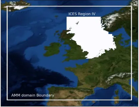
Fig. 1. The Atlantic Margin Model (AMM) boundary and the North Sea as defined by ICES region IV.

23

Fig. 1. The Atlantic Margin Model (AMM) boundary and the North Sea as defined by ICES region IV.

data there, but also because the North Sea is sufficiently dis-tant from the edge of the AMM domain that it should not suffer from open ocean boundary condition distortions. Fur-thermore, data-based validation of the POLCOMS-ERSEM model in the North Sea region is an important policy-driven task. Additionally, there was a computational upper limit on the size of the matching database; larger datasets covering large spatial regions required non-trivial computational re-sources.

The North Sea ICES region is defined as the sea between 62◦N and 51◦N, and 4◦W. The eastern boundary of the North Sea domain passes north from Agger Tange, Jutland, Denmark, to 57◦N, west to 8◦E, then north to 57◦300N, then west to 7◦_{E, then north to the coast of Norway.}

The in situ data were provided in a comma-separated-variable format, and contained a few data quality anoma-lies, such as repeated data, which were addressed during processing. The repeated measurements accounted for typ-ically 10–20 % of the database. Repeated data were iden-tified by searching for measurements with identical mea-surement time, longitude, latitude, depth and value. In some cases, data were recorded at depths much greater than the model bathymetry at the same point, so measurements with a depth greater than 5 m below the model bathymetry at the same point were ignored. The chlorophyll dataset contained a large proportion of measurements with a value of exactly 0.1, even at depths below 1 km. As no chlorophyll is ex-pected at large depths, this was interpreted to be the detec-tion limit of the database and all chlorophyll measurements below 100 m were removed from the study.

5 Methods

This section describes the methods that were used to test the compatibility of the model and the in situ data. The first sub-section describes how the point-to-point matching was ap-plied, the second the difference between time selection and time granularity, and the third the linear regression fit.

5.1 Point-to-point matching

The model and in situ datasets are intrinsically dissimi-lar. The model dataset is formed from a grid of continu-ous, evenly distributed, time-averaged cells of approximately 12 km by 12 km. The in situ dataset is a series of sporadic, un-evenly distributed, instantaneous measurements from a CTD or the mean of the contents of a sampling bottle. Further-more, the in situ measurements tended to occur at times and places which were readily accessible, convenient or well funded. These places and times do not match the uniform grid used by the model. The role of point-to-point matching was to reduce the impact of sampling bias when comparing these two distinct kinds of data.

The first step of the point-to-point matching process was performing a snap-to-grid: the in situ data were collected into the same grid cells as the model. Here, the full depth, daily mean, four-dimensional AMM domain grid was used. This grid had 40 depth layers, 198 longitude bins and 224 latitude bins per day. In the rare cases when multiple in situ measure-ments fell into the same three-dimensional grid cell on the same day, the mean of those measurements was used. Oth-erwise, the same model pixel could appear multiple times in the matched dataset.

Finally, all model pixels that did not have a corresponding in situ measurement were masked out and vice versa. In this way, no unpaired model or in situ data were used in the linear regression.

Techniques similar to this point-to-point matching have been used elsewhere in geoscientific models, but they are rare in marine ecosystem modelling. For instance, in J¨ockel et al. (2010), a dataset was created during the model run that matched a specific flight path with the highest model time resolution available. Similarly, in Lewis et al. (2006), Continuous Plankton Recorder tracks were extracted from a POLCOMS-ERSEM run for 1989–1990 in the North Sea. Unfortunately, the typical time required to produce a 45 yr POLCOMS-ERSEM hindcast is on the order of one month and implementing this technique could double the run time requirement. For this reason, run time methods of data recording were beyond the scope of this work.

(4)

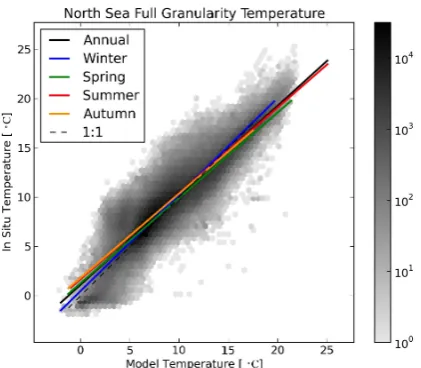
Fig. 2. Two-dimensional binned scatter plot of full granularity matched model data against in situ measurements for the North Sea temperature. The solid coloured lines show the linear regression fits for the full annual and seasonal data, and the dashed line is the line of unity slope that passes through the origin. The shading of the binned data density plot is scaled such that darker hue indicates logarithmically higher data density.

spatial scales than smaller ones for chlorophyll, with rela-tively poor skill when matching against satellite data on small spatial scales.

5.2 Time selection and granularity

It is important to highlight the difference between time selec-tion and time granularity. Once the matching was performed, both model and in situ datasets were studied under two time granularities: the annual mean and the daily mean. They were also studied under five different time selections: annual, win-ter, spring, summer and autumn. All ten permutations of the two granularities and the five time selections were studied.

The time granularity defines how that data are aggregated, if at all. The daily or “full” granularity refers to a dataset con-taining every matched pair of points in the North Sea, and the “annual” granularity is a series of annual means of that dataset. Typically, the full dataset contains many thousand matched pairs of in situ and model data, whereas the annual mean datasets contain only 35 points: one for every year be-tween 1970 and 2005. The annual time granularity allows the study of inter-annual variability in nature, in the model and in the sampling bias. The “full” granularity allows the com-parison of each in situ measurement to its model counterpart, and is used for identifying the limitations of the model.

The time selection specifies which part of the year is stud-ied. As the AMM is a Northern Hemisphere domain, the win-ter time selection masked out all measurements that did not occur in January, February or March. Similarly, the spring contains the data from April, May and June; the summer

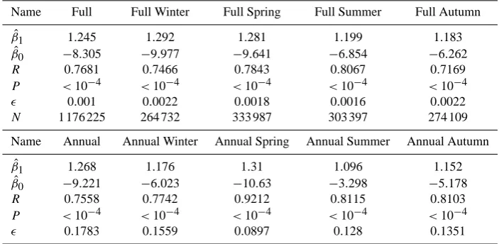
Fig. 3. Two-dimensional scatter plot of annual mean matched model data against in situ measurements for the North Sea temperature. The solid coloured lines show the linear regression fits for the an-nual and seasonal anan-nual means data, and the dashed line is the line of unity slope that passes through the origin. The matched seasonal means are shown as colour-coded scatter points.

contains the data from July, August and September; the au-tumn contains the data from October, November and Decem-ber. The annual time selection effectively means that no time selection was made and that data from all times of the year are used; it is sometimes referred to as “no time selection”.

As a shorthand, each combination of time selection and granularity can be described using the time granularity fol-lowed by the selection: for instance, full winter or annual spring. The specific case of the annual granularity and an-nual selection is called the anan-nual mean.

5.3 Linear regression

The relationship between model data and in situ measure-ments was plotted with the model on the x-axis and the in situ data on the y-axis, then fitted to a straight line using a least-squares linear regression. This technique minimises the sum of the square of the residuals; the residuals are the difference between a matched data pair and the closest point on the linear regression line. The five output parameters of the regression were the following: the y-axis intersect (_βˆ

0), the slope of the fit (_βˆ

(5)

Table 1. Linear regression output parameters for temperature.

Name Full Full Winter Full Spring Full Summer Full Autumn

ˆ

β1 0.9083 0.979 0.866 0.8704 0.8549

ˆ

β0 1.131 0.4908 1.28 1.701 1.83

R 0.9363 0.8637 0.894 0.9417 0.8598

P <10−4 <10−4 <10−4 <10−4 <10−4

0.0003 0.0011 0.0008 0.0006 0.001

N 1 191 530 271 599 334 676 308 946 276 309

Name Annual Annual Winter Annual Spring Annual Summer Annual Autumn

ˆ

β1 0.9565 1.192 0.9183 0.9101 0.8524

ˆ

β0 0.6754 −0.8403 0.8538 1.215 1.813

R 0.9572 0.9602 0.942 0.9814 0.9445

P <10−4 <10−4 <10−4 <10−4 <10−4

0.0469 0.0563 0.0531 0.0289 0.0481

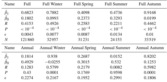
Table 2. Linear regression output parameters for salinity.

ˆ

β₁ 1.245 1.292 1.281 1.199 1.183

ˆ

β0 −8.305 −9.977 −9.641 −6.854 −6.262

R 0.7681 0.7466 0.7843 0.8067 0.7169

P <10−4 <10−4 <10−4 <10−4 <10−4

0.001 0.0022 0.0018 0.0016 0.0022

N 1 176 225 264 732 333 987 303 397 274 109

ˆ

β1 1.268 1.176 1.31 1.096 1.152

ˆ

β0 −9.221 −6.023 −10.63 −3.298 −5.178

R 0.7558 0.7742 0.9212 0.8115 0.8103

P <10−4 <10−4 <10−4 <10−4 <10−4

0.1783 0.1559 0.0897 0.128 0.1351

output parameters are correct, under the assumption that all data points have an equal influence on the fit. As such, given a matched dataset with some relationship between the in situ and the model, thepvalue tends to decrease with large sam-ple size, even when the relationship is weak or non-linear.

6 Results

The results of the linear regression fits are shown in Tables 1– 5. These tables hold the results of the linear regression for the North Sea temperature (T), salinity (Sal.), nitrates (NO3), phosphates (PO4) and chlorophyll (Chl.) datasets. Each table contains both the full and the annual time granularity for each of the five time selections, as described in Sect. 5.2. The rows of these tables contain the five output parameters of the re-gression: the slope of the fit (βˆ1), the y-axis intersect (βˆ0), the correlation coefficient (R), the two-tailed probability (P), the

standard error (), and the number of data in the sample (N). The number of data in the sample,N, is the total number of data pairs that contributed to the linear regression. However, in the case of the annual means, the number of entries that were regressed is 35 or less, equivalent to one entry for each year (1970–2005), andN is not shown.

(6)

Table 3. Linear regression output parameters for nitrates.

ˆ

β1 1.05 1.267 0.9105 0.6153 0.8885

ˆ

β0 −4.248 −8.121 −1.355 −1.016 −3.409

R 0.5928 0.6584 0.4567 0.3728 0.5548

P <10−4 <10−4 <10−4 <10−4 <10−4

0.0042 0.0082 0.0102 0.0101 0.0074

N 116 933 31 575 30 243 22 892 32 223

ˆ

β1 0.6872 1.336 0.6463 0.6168 0.7163

ˆ

β0 0.2063 −10.05 0.9477 −0.8275 −0.843

R 0.8132 0.8191 0.7484 0.5798 0.7207

P <10−4 <10−4 <10−4 0.0001 <10−4

0.0798 0.1518 0.0929 0.1406 0.1118

Table 4. Linear regression output parameters for phosphates.

ˆ

β₁ 0.6823 0.7882 0.4098 0.4736 0.9168

ˆ

β0 0.1802 0.0993 0.2373 0.3293 0.0199

R 0.4153 0.4926 0.2583 0.2211 0.4462

P <10−4 <10−4 <10−4 <10−4 <10−4

0.0043 0.0077 0.0087 0.0134 0.01

N 121 860 32 957 31 231 24 153 33 519

ˆ

β1 0.1814 0.938 0.2687 0.0152 0.8202

ˆ

β0 0.4929 −0.0255 0.3015 0.532 0.1253

R 0.1283 0.5799 0.2179 0.0082 0.5982

P 0.43 0.0001 0.1769 0.9598 0.0001

0.2274 0.2167 0.1952 0.2991 0.1806

the top left region and overestimates the in situ data in the lower right region. In addition to the lines of best fit for the full granularities, Figs. 2, 4, 6, 8 and 10 also show the full granularity matched data as a binned scatter plot. The shad-ing of the binned scatter plots is scaled such that darker hue indicates logarithmically higher data density. However, the linear regression fits were performed using a non-logarithmic scale. Figures 3, 5, 7, 9 and 11 show the linear regressions for each annual granularity time selection and also contain colour-coded scatter plots of the annual means for each of the four seasons.

The linear regression lines in Figs. 2–11 were drawn with a horizontal and vertical range between the smallest and largest value of either the matched model or the in situ data. This method makes comparison between time selections relatively straightforward, but it can sometimes be misleading. For in-stance, the darker high density regions of Figs. 2, 4, 6, 8 and

10 all coincide with the line of best fit and the line of slope unity through the origin. However, the best fit lines appear to diverge from the matched points in the lower data density regions.

(7)

Table 5. Linear regression output parameters for chlorophyll.

ˆ

β1 0.7479 0.8829 0.5341 0.9941 3.391

ˆ

β0 2.052 1.165 2.952 1.98 0.7616

R 0.2379 0.2132 0.186 0.23 0.2609

P <10−4 <10−4 <10−4 <10−4 <10−4

0.0171 0.05 0.0264 0.0418 0.2

N 32 019 6552 11 406 10 121 3940

ˆ

β1 1.098 0.1448 1.62 3.031 4.514

ˆ

β0 1.139 1.839 0.2675 −0.0887 0.7984

R 0.2844 0.0632 0.37 0.7083 0.3444

P 0.0793 0.7492 0.0263 <10−4 0.0674

0.6085 0.4483 0.6975 0.5515 2.369

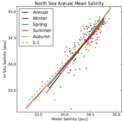
Fig. 4. Two-dimensional binned scatter plot of full granularity matched model data against in situ measurements for the North Sea salinity. The solid coloured lines show the linear regression fits for the full annual and seasonal data, and the dashed line is the line of unity slope that passes through the origin. The shading of the binned data density plot is scaled such that darker hue indicates logarithmi-cally higher data density.

marine models tend to be more successful at simulating physics than biology, temperature is the variable where the best correlation is expected. Furthermore, ocean temperature has much less variability over small temporal and spatial scales than the biological observables.

The salinity plots in Figs. 4 and 5 show good agreement between in situ and model for the regions of high density, and that these regions coincide with the line of slope unity through the origin. These plots are a good example of how the difference between the ranges of the full and the annual

Fig. 5. Two-dimensional scatter plot of annual mean matched model data against in situ measurements for the North Sea salinity. The solid coloured lines show the linear regression fits for the annual and seasonal annual means data, and the dashed line is the line of unity slope that passes through the origin. The matched seasonal means are shown as colour-coded scatter points.

plots impacts the perceived model quality. The full in situ data range between 0 and 36 psu, whereas the annual mean data has a much tighter range between 33 and 35 psu. This indicates that the bulk of the in situ data are well matched, even though a cursory glance at Fig. 4 might give the oppo-site impression.

(8)

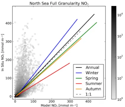
Fig. 6. Two-dimensional binned scatter plot of full granularity matched model data against in situ measurements for the North Sea nitrates. The solid coloured lines show the linear regression fits for the full annual and seasonal data, and the dashed line is the line of unity slope that passes through the origin. The shading of the binned data density plot is scaled such that darker hue indicates logarithmi-cally higher data density.

Fig. 7. Two-dimensional scatter plot of annual mean matched model data against in situ measurements for the North Sea nitrates. The solid coloured lines show the linear regression fits for the annual and seasonal annual means data, and the dashed line is the line of unity slope that passes through the origin. The matched seasonal means are shown as colour-coded scatter points.

of the measurements. For instance, at the confluence of a river and the sea, the salinity may range from nearly 0 psu near the river mouth to 35 psu 10 km away in the sea. How-ever, this model has 12 km by 12 km pixel size, and all mea-surement data between the river mouth and 10 km offshore

Fig. 8. Two-dimensional binned scatter plot of full granularity matched model data against in situ measurements for the North Sea phosphates. The solid coloured lines show the linear regression fits for the full annual and seasonal data, and the dashed line is the line of unity slope that passes through the origin. The shading of the binned data density plot is scaled such that darker hue indicates logarithmically higher data density.

Fig. 9. Two-dimensional scatter plot of annual mean matched model data against in situ measurements for the North Sea phosphates. The solid coloured lines show the linear regression fits for the annual and seasonal annual means data, and the dashed line is the line of unity slope that passes through the origin. The matched seasonal means are shown as colour-coded scatter points.

(9)

Fig. 10. Two-dimensional binned scatter plot of full granularity matched model data against in situ measurements for the North Sea chlorophyll. The solid coloured lines show the linear regression fits for the full annual and seasonal data, and the dashed line is the line of unity slope that passes through the origin. The shading of the binned data density plot is scaled such that darker hue indicates logarithmically higher data density.

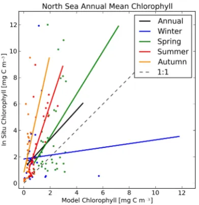
Fig. 11. Two-dimensional scatter plot of annual mean matched model data against in situ measurements for the North Sea chloro-phyll. The solid coloured lines show the linear regression fits for the annual and seasonal annual means data, and the dashed line is the line of unity slope that passes through the origin. The matched seasonal means are shown as colour-coded scatter points.

By using the point-to-point matching method, it becomes possible to identify some limitations of the model. For in-stance, the off-diagonal regions of the salinity, nitrates and phosphates full data density plots in Figs. 4, 6 and 8 con-tain significantly fewer data than the densely populated

Fig. 12. Annual North Sea temperature time series plot: the black line is the matched model mean annual temperature, the dashed line the annual mean in situ temperature, and and the grey line shows the MLD-averaged mean temperature of the North Sea.

on-diagonal hot spots. However, the presence of any points at all away from the dashed line indicates that the model did not accurately reproduce all the in situ measurements. The model overestimated the salinity of many freshwater in situ measurements and underestimated many of the in situ mea-surements with high nitrates and phosphates. In both cases, the model predicted a value less extreme than the outly-ing in situ measurement. Some of these discrepancies can be explained as an effect of the high spatial variability in salinity and nitrates in the well-sampled coastal and river-influenced regions against the relatively low spatial resolu-tion of the model. In addiresolu-tion, the in situ data are of instan-taneous character, while the model data are a daily average, further enhancing the in situ measurement variability. Con-versely, Figs. 4, 6 and 8 all contain a small number of points where the opposite situation occurred: the model salinity was underestimated, and the nitrate and phosphate concentrations were overestimated. These data suggest that there may be some events in the river forcing where the model has a larger influx of fresh water and nutrients than was observed in na-ture.

The seasonal nitrate and phosphate scatter plots in Figs. 7 and 9 shows that the model captures the seasonality of the nutrient cycle with winter peaks and a spring and summer depletion. However, it is important to bear in mind that these data are not indicative of the mean state of the system. Rather, these figures indicate that the nutrient seasonality is apparent in both model and data despite the data used being an arbi-trary subsection of measurements of the North Sea.

(10)

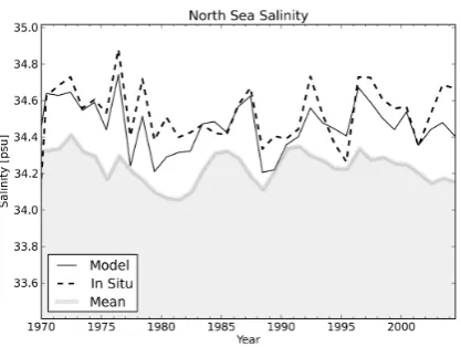
Fig. 13. Annual North Sea salinity time series: the black line is the matched model mean annual salinity, the dashed line the mean annual in situ salinity, and the grey area shows the MLD-averaged mean salinity of the North Sea.

Fig. 14. North Sea mean winter nitrates time series: the black line is the matched model mean winter nitrates, the dashed line the mean winter in situ nitrates, and the grey area shows the MLD-averaged mean nitrate of the North Sea.

the densely populated on-diagonal hot spots, but also has a region where the model overestimates the in situ chlorophyll. A significant difference between the full and the annual data appears in Figs. 10 and 11. The full plot (Fig. 10) shows that the spring, winter and annual model data tend to overes-timate the in situ chlorophyll in the fit, while the summer fit is close to the 1:1 line. However, the annual mean chlorophyll plot (Fig. 11) indicates that the annual, autumn, summer and spring chlorophyll are underestimated by the model. Once again, it is important to remember that the in situ dataset, and hence the model data, is an arbitrary subsection of the North Sea.

The ICES chlorophyll database has been amalgamated from a wide selection of sources, using multiple measure-ment techniques, whose uncertainties vary from more to less validated. Of the five datasets studied here, chlorophyll

Fig. 15. North Sea mean winter phosphates time series: the black line is the matched model mean winter phosphates, the dashed line the mean winter in situ phosphates, and the grey area shows the MLD-averaged mean phosphates of the North Sea.

typically has the highest measurement uncertainty. Addition-ally, in order for a model to capture the phytoplankton be-haviour, it must first model the physics and nutrient dynamics appropriately. The model errors and uncertainties are com-pounded with each step away from a tractable physics ob-servable towards the biological end of the model. As such, chlorophyll is the dataset with the highest in situ measure-ment uncertainty and with the highest model uncertainty. While there is not an excellent agreement between model and the in situ chlorophyll in Figs. 10 and 11, there is a good enough agreement.

(11)

Fig. 16. North Sea mean spring chlorophyll time series: the black line is the matched model mean spring chlorophyll, the dashed line the mean spring in situ chlorophyll, and the grey area shows the MLD-averaged mean chlorophyll of the North Sea.

the matched model data and the in situ measurements, espe-cially in the case of nitrates, phosphates and chlorophyll in Figs. 14–17.

The results of the linear regressions of Figs. 12–17 are shown in Tables 6 and 7. These tables have two columns: the results of the linear regression of the MLD-averaged model data against the in situ, and the linear regression of the matched data against the in situ data. In all cases shown here, the matching resulted in a higher correlation coefficient, decreasedpvalue, and they-intersect closer to zero. In all cases shown except summer chlorophyll, matching results in a slope closer to unity than the MLD-averaged linear regres-sion. The fit for each dataset is discussed in more detail be-low.

Figure 12 is a time-series plot of the annual mean North Sea temperature. The mean of the MLD-averaged data is the depth-averaged temperature, but the matched data and in situ measurements may be from any depth. For this rea-son, the MLD-averaged mean model temperature was consis-tently higher than the in situ and the mean matched temper-ature. This shift is also visible in the difference in the slope andy-intersect,βˆ1andβˆ0, in Table 6. As the model surface temperature is forced using reanalysis based on aggregated observational data, it is not surprising that the temperature in Table 1 shows a strong correlation between the model and the in situ data. However, the atmospheric forcing dataset, ERA40-reanalysis (Uppala et al., 2005), is a meteorological surface dataset, whereas the in situ measurements and hence the matched model data may occur at any depth. As such, the success of the model is due to its own merit, instead of the similarities between the forcing and in situ datasets. Both the matched model and the MLD-averaged data capture the 1990 in situ peak and subsequent rise in Fig. 12. This sug-gests that some of the increase seen in the mean in situ tem-perature between 1993 and 2005 is not an artefact of uneven

Fig. 17. North Sea mean summer chlorophyll time series: the black line is the matched model mean summer chlorophyll, the dashed line the mean summer in situ chlorophyll, and the grey area shows the MLD-averaged mean chlorophyll of the North Sea.

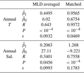
Table 6. Linear regression output parameters for temperature (T) and salinity (Sal.). The parameters shown are the slope of the line (_βˆ

1), the y-axis intersect (βˆ0), the correlation coefficient (R), and the two-tailed probability (P), the standard error (), and the num-ber of data (N).

MLD averaged Matched

ˆ

β₁ 0.4495 0.9565

Annual _βˆ

0 6.02 0.6754

T R 0.643 0.9572

P <10−4 <10−4

0.0932 0.0469

ˆ

β1 0.2063 1.268

Annual βˆ0 27.11 −9.221

Sal. R 0.3401 0.7558

P 0.0456 <10−4

0.0993 0.1783

sampling, but rather physically observable inter-annual vari-ability.

(12)

Table 7. Linear regression output parameters for nitrates (NO3), phosphates (PO4) and chlorophyll (Chl.). The parameters shown are the slope of the line (_βˆ

1), the y-axis intersect (βˆ0), the correlation coefficient (R), and the two-tailed probability (P), the standard er-ror (), and the number of data (N).

MLD averaged Matched

ˆ

β1 0.0295 1.336

Winter βˆ0 13.64 −10.05

NO3 R 0.3781 0.8191

P 0.0251 <10−4

0.0126 0.1518

ˆ

β1 0.0229 0.938

Winter βˆ0 0.7217 −0.0255

PO4 R 0.1602 0.5799

P 0.3654 0.0001

0.0249 0.2167

ˆ

β1 0.007 1.62

Spring _βˆ

0 1.966 0.2675

Chl. R 0.1473 0.37

P 0.4212 0.0263

0.0085 0.6975

ˆ

β1 −0.0113 3.031

Summer _βˆ

0 0.7444 −0.0887

Chl. R −0.5414 0.7083

P 0.002 <10−4

0.0033 0.5515

The mean winter North Sea nitrates are shown in Fig. 14, and the mean winter North Sea phosphates are shown in Fig. 15. These plots show that the model had significant skill in reproducing the in situ nitrate and phosphate mea-surements, but only once unpaired model cells were masked. The winter nitrate linear regression fit was consistent with a line of unity slope, and had a correlation coefficient of R=0.8191. This correlation was not present in the un-matched mixed layer depth-averaged model nitrates in Ta-ble 3 or Fig. 14, suggesting that the bulk of the inter-annual variability of in situ nitrates is a result of sampling. The other time selections and granularities of the nitrates in Table 3 in-dicate that the inter-annual variability of in situ nitrates was reasonably reproduced under other time granularities and se-lections. However, the winter nutrient behaviour is arguably more important than the rest of the years as the winter nu-trients determine the resources available for the spring phy-toplankton bloom. The winter phosphate linear regression fit was consistent with a line of unity slope and a null inter-sect, but this skill was not present in the spring and summer phosphates in Table 4. The annual summer phosphate col-umn of this table shows an instance of the model and the in situ data match breaking down; the correlation and slope are both very close to zero, and thepvalue is nearly unity. How-ever, the nutrients are depleted in the summer, and the results

P

ap

er

|

Disussion

P

ap

er

|

Disussion

P

ap

er

|

Disussion

P

ap

er

|

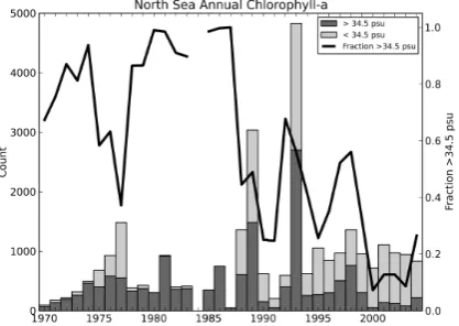
Fig. 18. The number of North Sea in situ Chlorophyll measurements, grouped into a high salinity (Sal.> 34.5PSU) in dark grey and low salinity (Sal.<34.5PSU) in light grey. The dark line shows the fraction of high salinity. ] There is a gap in 1984 due the absence of simultaneous measurements of Chlorophyll and salinity.

40

Fig. 18. The number of North Sea in situ chlorophyll measurements, grouped into a high salinity (Sal.>34.5 psu) in dark grey and low salinity (Sal.<34.5 psu) in light grey. The dark line shows the frac-tion of high salinity. There is a gap in 1984 due to the absence of simultaneous measurements of chlorophyll and salinity.

of a linear regression would be skewed towards large outly-ing in situ measurements, which would never be reproduced by the model. Secondly, winter phosphate has a much larger impact on the ecosystems annual cycle, and its successful simulation by the model has more importance.

Figures 14 and 15 both show a large peak in 1983. In the winter of 1983, almost all North Sea nitrate and phosphate measurements in the ICES database were taken in coastal en-vironments. The peaks are also present in the matched model data, but not in the mean of the MLD-averaged nitrates and phosphates. The presence of these peaks in both model and measurement suggests that the bulk of the variability of in situ nitrates and phosphates is due to uneven coverage, rather than inter-annual variability. Due to the incongruities of his-toric in situ data such as these peaks, model validators should be extremely cautious to ensure that their validation com-pares like-datasets to each other.

(13)

P

ap

er

|

Disussion

P

ap

er

|

Disussion

P

ap

er

|

Disussion

P

ap

er

|

Fig. 19. Target diagram showing the impact of the transition from the unmatched to the matched methods on temperature.

41

Fig. 19. Target diagram showing the impact of the transition from the unmatched to the matched methods on temperature.

chlorophyll data after 1993 was measured where the model is less effective.

Despite these limitations, the matched model data repro-duced the variability of the in situ chlorophyll measurements with a correlation ofR=0.708 in the annual summer. The matched model data did not produce a significant correla-tion with the spring in situ data. This can be explained by the greater chlorophyll variability in the spring, and the high sensitivity to bloom timing. A small difference in the model bloom timing relative to nature will result in a large resid-ual. Additionally, as the seasons were defined as strict three-month periods, it is possible that, for the earliest blooms, for instance in a coastal area, the springtime bloom may have overflowed into the wintertime bin. This bin edge over-flow is a more critical issue for chlorophyll linear regression due to its rapid blooms than for temperature, which is much smoother. It is also possible that some of the in situ chloro-phyll measurements were biased towards regions that were biologically active.

Although much of the in situ variability of the larger datasets (temperature, salinity, nitrates, and phosphates) can be accounted for by the model, POLCOMS-ERSEM does not reproduce many of the historic trends of the in situ chloro-phyll measurements on a point-to-point basis. While a more diverse distribution of North Sea chlorophyll measurements would help to validate the model or produce new biogeo-chemical parametrisations, it is not possible to travel back in time to obtain such a dataset. The failure to reproduce the his-toric data time series may be due to the effects of sub-pixel variability, in which case higher resolution models could al-low a point-to-point study of chlorophyll to converge on the in situ measurements. It is also possible that a better match between the in situ measurements and the model may yet

P

ap

er

|

Disussion

P

ap

er

|

Disussion

P

ap

er

|

Disussion

P

ap

er

|

Fig. 20. Target diagram showing the impact of the transition from the unmatched to the matched methods on salinity.

42

Fig. 20. Target diagram showing the impact of the transition from the unmatched to the matched methods on salinity.

Disussion

P

ap

er

|

Disussion

P

ap

er

|

Disussion

P

ap

er

|

Disussion

P

ap

er

|

Fig. 21. Target diagram showing the impact of the transition from the unmatched to the matched methods on nitrates.

43

Fig. 21. Target diagram showing the impact of the transition from the unmatched to the matched methods on nitrates.

occur through improvements to the phytoplankton parametri-sation.

(14)

P

ap

er

|

Disussion

P

ap

er

|

Disussion

P

ap

er

|

Disussion

P

ap

er

|

Fig. 22. Target diagram showing the impact of the transition from the unmatched to the matched methods on phosphates.

44

Fig. 22. Target diagram showing the impact of the transition from the unmatched to the matched methods on phosphates.

Figures 19–23 are target diagrams (Jolliff et al., 2009) showing the pattern statistics for each of the five datasets. The x-axis shows the normalised unbiased root mean square difference (RMSD0), and the y-axis shows the normalised bias. Normalisation is performed by dividing by the refer-ence standard deviation,σref, which is the standard deviation of the in situ data. The diagram’s two large circles correspond to lines of constant root mean square difference (RMSD): the outer has RMSD=1.0, and the dashed inner circle has an RMSD=0.71. In these plots, the square markers describe the comparison of the MLD-averaged data to the mean of the in situ data (unmatched). The round markers are the pattern statistics of the matched model data against the mean of the in situ data (matched). The grey arrows indicate the change due to moving the unmatched to the matched methods. In all the target diagrams, the annual mean time granularity was used because of the absence of the MLD-averaged data with full time granularity. The colour scale of the markers shows the correlation coefficient. As with most targets, the best out-comes occur closer to the centre of the target.

Figures 19 and 20 are concise plots showing change due to the application of the matching method to temperature and salinity data. Reflecting the conclusions of Figs. 12 and 13, the matching significantly improved the correlation, and the normalised bias and RMSD0_{, moving all temperature and}

salinity markers closer to the centre. The salinity target dia-gram is particularly impressive as it shows a large decrease in the bias, and a large increase in correlation due to going from an unmatched comparison to a point-to-point comparison.

Although winter nitrates in Fig. 21 show the best improve-ment in bias and RMSD of that figure, all time selections show unambiguous increases in correlation, shifting from cold colours to hot colours. The other time selections also

P

ap

er

|

Disussion

P

ap

er

|

Disussion

P

ap

er

|

Disussion

P

ap

er

|

Fig. 23. Target diagram showing the impact of the transition from the unmatched to the matched methods on chlorophyll-a.

45

Fig. 23. Target diagram showing the impact of the transition from the unmatched to the matched methods on chlorophylla.

show substantial shifts; the markers move across the diagram while maintaining an approximately constant RMSD.

In Fig. 22, the autumn and winter phosphate time se-lections both moved inside the RMSD=1.0 circle and in-creased in correlation. The other phosphate time selections maintained similar unbiased RMSD0 while decreasing their normalised bias.

In terms of the chlorophylla, Fig. 23 shows that match-ing does not produce the dramatic shifts seen in the other measurements. However, it is clear from the legend that the match increased the chlorophyll correlation, except for in the winter. The normalised bias decreased in all time selections, and the unbiased RMSD0decreased in all time selections but winter.

(15)

7 Conclusions

A point-to-point method was presented as a tool to validate a marine biogeochemical model hindcast of the POLCOMS-ERSEM model with sparse historic CTD and low-resolution bottle in situ measurements. To demonstrate the method, in situ temperature, salinity, nitrates, phosphates, and chloro-phyll a from the North Sea were compared against both the point-to-point model data and the annual and seasonal means.

Firstly, the point-to-point method was used to show that POLCOMS-ERSEM displayed skill at reproducing all five of the variables. POLCOMS-ERSEM is most successful at reproducing the physical variables (temperature and salinity) and is least successful at reproducing the biological variable chlorophyll on a pixel by pixel basis. The model had mod-erate skill at reproducing the nutrients phosphate and nitrate, especially in the winter. This is to be expected, as the physical variables are relatively deterministic, tractable and straight-forward to calculate. While the chlorophyll in situ dataset was only reproduced with moderate success, due to the com-plex and highly variable biological network, even modest success at reproducing chlorophyll trends should be heralded as a victory.

Secondly, using time series plots, it was shown that POLCOMS-ERSEM has significant skill in reproducing the inter-annual variability of some policy-driven time selections of in situ datasets. It also became apparent that the bulk of the variability in the in situ measurements may be due to uneven and low coverage, rather than inter-annual variability of the mean state of the system. For these reasons, we recommend that in situ datasets such as these should be used with caution in trend and inter-annual variability studies.

Thirdly, target diagrams were used to identify some of the strengths and weaknesses of the matching method. It was found that the matching method does not always pro-duce simultaneous improvements to bias, root mean square difference and correlation. However, improvements in bias, RMSD0and correlation relative to the unmatched model were observed in most cases studied here. These improvements are not guaranteed nor are they the principal motivation for the use of the point-to-point method. The point-to-point method is simply a better method to exploit sparse, uneven in situ data while compensating for its variability.

The ICES datasets have been shown to be useful for model validation, and their limitations do not hinder point-to-point matching. Nevertheless, there is a need for larger and longer term non-coastal datasets, which could perhaps be fulfilled in part through the use of next-generation Bio-Argo floats or wave gliders. In addition to validating the model ability, these datasets are required to understand model behaviour and, consequently, to plan next-generation model develop-ment and validation. Future in situ datasets should strive for consistent multi-decadal coverage and good representation of both coastal and offshore environments.

Finally, it is important to remember that historic datasets were not recorded for the purpose of model validation; they have limits. As such, it is crucial to account for these restric-tions when validating hindcasts. When performing a model validation using a direct comparison, it is necessary to pro-cess the model data to resemble the in situ dataset as much as possible. If a direct comparison validation is performed without some kind of matching, the predictive power of the model could be seriously misjudged.

Acknowledgements. This work is supported by the NERC National Capability in Modelling programme at Plymouth Marine Labora-tory and Theme 6 of the EC seventh framework program through the Marine Ecosystem Evolution in a Changing Environment (MEECE No. 212085) Collaborative Project.

Edited by: A. Stenke

References

Arhonditsis, G. B. and Brett, M. T.: Evaluation of the current state of mechanistic aquatic biogeochemical modelling, Mar. Ecol. Prog. Ser., 271, 13–26, doi:10.3354/meps271013, 2004.

Blackford, J. C., Allen, J. I., and Gilbert, F. J.: Ecosystem dynam-ics at six contrasting sites: a generic modelling study, J. Marine Syst., 52, 191–215, doi:10.1016/j.jmarsys.2004.02.004, 2004. Doney, S. C., Lima, I., Moore, J. K., Lindsay, K.,

Behren-feld, M. J., Westberry, T. K., Mahowald, N., Glover, D. M., and Takahashi, T.: Skill metrics for confronting global up-per ocean ecosystem-Biogeochemistry models against field and remote sensing data, J. Marine Syst., 76, 95–112, doi:10.1016/j.jmarsys.2008.05.015, 2009.

Edwards, K. P., Barciela, R., and Butensch¨on, M.: Validation of the NEMO-ERSEM operational ecosystem model for the North West European Continental Shelf, Ocean Sci., 8, 983–1000, doi:10.5194/os-8-983-2012, 2012.

FAO: FAO Major Fishing Areas, (Major Fishing Area 27), CWP Data Collection, available at: http://www.fao.org/fishery/area/ Area27/en#NB04F5, (last access: 17 August 2012), 2008. Garcia, H. E. and Levitus, S.: World Ocean Atlas 2005, vol. 4,

Nutrients (phosphate, nitrate, silicate), Tech. Rep. 64, National Oceanographic Data Centre (US), Ocean Climate Laboratory, Washington, DC, 2010a.

Garcia, H. E. and Levitus, S.: World Ocean Atlas 2005, vol. 3, Dis-solved oxygen, apparent oxygen utilisation, and oxygen satura-tion, Tech. Rep. 63, National Oceanographic Data Centre (US), Ocean Climate Laboratory, Washington, DC, 2010b.

Holt, J., James, I. D., and Jones, J. E.: An s coordinate density evolv-ing model of the northwest European continental shelf 2, Sea-sonal currents and tides, J. Geophys. Res., 106, 14035–14053, doi:10.1029/2000JC000303, 2001.

(16)

ICES: ICES Dataset on Ocean Hydrography, The International Council for the Exploration of the Sea Copenhagen, Copen-hagen, 2009.

J¨ockel, P., Kerkweg, A., Pozzer, A., Sander, R., Tost, H., Riede, H., Baumgaertner, A., Gromov, S., and Kern, B.: Development cycle 2 of the Modular Earth Submodel System (MESSy2), Geosci. Model Dev., 3, 717–752, doi:10.5194/gmd-3-717-2010, 2010. Jolliff, J. K., Kindle, J. C., Shulman, I., Penta, B., Friedrichs, M. A.,

Helber, R., and Arnone, R. A.: Summary diagrams for cou-pled hydrodynamic-ecosystem model skill assessment, J. Marine Syst., 76, 64–82, doi:10.1016/j.jmarsys.2008.05.014, 2009. Lewis, K., Allen, J., Richardson, A. J., and Holt, J.: Error

quantification of a high resolution coupled hydrodynamic-ecosystem coastal-ocean model: Part 3, validation with con-tinuous plankton recorder data, J. Marine Syst., 63, 209–224, doi:10.1016/j.jmarsys.2006.08.001, 2006.

OSPAR Commission: Common Procedure for the Identification of the Eutrophication Status of the OSPAR Maritime Area, UK Na-tional Report, London, UK, 2008.

Robeson, S.: Influence of spatial sampling and interpolation on es-timates of air temperature change, Clim. Res., 4, 119–126, 1994. Saux Picart, S., Butensch¨n, M., and Shutler, J. D.: Wavelet-based spatial comparison technique for analysing and evaluating two-dimensional geophysical model fields, Geosci. Model Dev., 5, 223–230, doi:10.5194/gmd-5-223-2012, 2012.

Stow, C. A., Jolliff, J., Mcgillicuddy, D. J., Doney, S. C., Allen, J. I., Friedrichs, M. A. M., Rose, K. A., and Wallhead, P.: Skill assess-ment for coupled biological/physical models of marine systems, J. Marine Syst., 76, 4–15, doi:10.1016/j.jmarsys.2008.03.011, 2009.

Taylor, K. E.: Summarizing multiple aspects of model performance in a single diagram, J. Geophys. Res., 106, 7183–7192, 2001. Uppala, S. M., K ˚Allberg, P. W., Simmons, A. J., Andrae, U.,

Bech-told Da Costa, V., Fiorino, M., Gibson, J. K., Haseler, J., Her-nandez, A., Kelly, G. A., Li, X., Onogi, K., Saarinen, S., Sokka, N., Allan, R. P., Andersson, E., Arpe, K., Balmaseda, M. A., Beljaars, A. C. M., Berg, L. Van De, Bidlot, J., Bormann, N., Caires, S., Chevallier, F., Dethof, A., Dragosavac, M., Fisher, M., Fuentes, M., Hagemann, S., H´olm, E., Hoskins, B. J., Isaksen, L., Janssen, P. A. E. M., Jenne, R., Mcnally, A. P., Mahfouf, J.-F., Morcrette, J.-J., Rayner, N. A., Saunders, R. W., Simon, P., Sterl, A., Trenberth, K. E., Untch, A., Vasiljevic, D., Viterbo, P., and Woollen, J.: The ERA-40 re-analysis, Q. J. Roy. Meteorol. Soc., 131, 2961–3012, doi:10.1256/qj.04.176, 2005.

V¨or¨osmarty, C. J., Fekete, B. M., Meybeck, M., and Lam-mers, R. B.: Global system of rivers: its role in organizing con-tinental land mass and defining land-to-ocean linkages, Global Biogeochem. Cy., 14, 599–621, doi:10.1029/1999GB900092, 2000.