Iranian Journal of Mathematical Sciences and Informatics Vol. 13, No. 1 (2018), pp 111-129
DOI: 10.7508/ijmsi.2018.1.011
A New High Order Closed Newton-Cotes
Trigonometrically-fitted Formulae for the Numerical Solution
of the Schr¨
odinger Equation
Ali Shokri∗, Hosein Saadat, Alireza Khodadadi
Department of Mathematics, Faculty of Basic Science, University of Maragheh, P.O. Box 55181-83111, Maragheh, Iran.
E-mail: [email protected] E-mail: [email protected] E-mail: ali−reza−[email protected]
Abstract. In this paper, we investigate the connection between closed Newton-Cotes formulae, trigonometrically-fitted methods, symplectic
in-tegrators and efficient integration of the Schr¨odinger equation. The study
of multistep symplectic integrators is very poor although in the last
decades several one step symplectic integrators have been produced based
on symplectic geometry (see the relevant literature and the references
here). In this paper, we study the closed Newton-Cotes formulae and
we write them as symplectic multilayer structures. Based on the closed
Newton-Cotes formulae, we also develop trigonometrically-fitted
symplec-tic methods. An error analysis for the one-dimensional Schr¨odinger
equa-tion of the new developed methods and a comparison with previous
de-veloped methods is also given. We apply the new symplectic schemes to
the well-known radial Schr¨odinger equation in order to investigate the
efficiency of the proposed method to these type of problems.
Keywords: Phase-lag, Schr¨odinger equation, Numerical solution, Newton-Cotes formulae, Derivative.
∗Corresponding Author
Received 04 October 2015; Accepted 30 April 2016 c
2018 Academic Center for Education, Culture and Research TMU
111
2000 Mathematics subject classification: 65L05, 65L06, 65L20. 1. Introduction
It is of great interest the research area of development of numerical inte-gration methods for ordinary differential equations that preserve qualitative properties of the analytic solution. In this paper, we consider Hamilton equa-tions of motion which are linear in positionpand momentumq
˙ q=mp
˙
p=−mq (1.1)
wherem is a constant scalar or matrix. The Eq. (1.1) is an important one in the field of molecular dynamics.
In order to preserve the characteristics of the Hamiltonian system in the numerical approximation, it is necessary to use symplectic integrators. In the recent years work has been done mainly in the production of one step symplec-tic integrators (see [1]). Zhu et al. [26] have studied the symplecsymplec-tic integrators and the well-known open Newton-Cotes differential methods. They have pre-sented the open Newton-Cotes differential methods as multilayer symplectic integrators. The construction of multistep symplectic integrators based on the open Newton-Cotes integration methods was investigated by Chiou and Wu [2]. The last decades much work has been done on exponential and trigono-metrically fitting and the numerical solution of periodic initial value problems (see [3-20] and references therein). In this paper:
•We try to present closed Newton-Cotes differential methods as multilayer symplectic integrators.
• We apply the closed Newton-Cotes methods on the Hamiltonian system (1) and we obtain the result that the Hamiltonian energy of the system remains almost constant as the integration proceeds.
•The trigonometrically-fitted methods are developed.
•An error analysis for the one-dimensional Schr¨odinger equation of the new developed methods and a comparison with previous developed methods is also given.
We note that the aim of this paper is to generate methods that can be used for non-linear differential equations as well as linear ones. In Section 2 the re-sults about symplectic matrices and schemes are presented. In Section 3 closed Newton-Cotes integral rules and differential methods are described and the new trigonometrically-fitted methods are developed. In Section 4 the conver-sion of the closed Newton-Cotes differential methods into multilayer symplectic structures is presented. The error analysis for the one-dimensional Schr¨odinger equation of the new developed methods and a comparison with previous devel-oped methods is presented in Section 5. Finally, numerical results are presented in Section 6.
2. Basic Theory on Symplectic Schemes and Numerical Methods Zhu et al. [26] have obtained a theory on symplectic numerical schemes and symplectic matrices in which the following basic theory is based.
Dividing an interval [a, b] withN points we have
x0=a , xn=x0+nh=b, n= 1,2,· · ·, N (2.1) The above division leads to the following discrete scheme:
p n+1 qn+1
=Mn+1
p n
qn
, Mn+1=
an+1 bn+1
cn+1 dn+1
!
. (2.2)
We note thatxis the independent variable andaandbin the equation forx0 (Eq. (2.1)) are different than theaandbin Eq. (2.2). Based on the above we can write the n-step approximation to the solution as
p n
qn
= an bn cn dn
!
an−1 bn−1
cn−1 dn−1
!
· · · a1 b1 c1 d1
! p
0 q0
= MnMn−1, . . . , M1
p0 q0
.
Defining
S=MnMn−1, . . . , M1=
An Bn
Cn Dn !
the discrete transformation can be written as
p n+1 qn+1
=S
p
0 q0
.
A discrete scheme (2.2) is a symplectic scheme if the transformation matrix S is symplectic. A matrix A is symplectic ifATJ A=J where
J = 0 1 −1 0
!
The product of symplectic matrices is also symplectic. Hence, if each matrix Mnis symplectic the transformation matrixSis symplectic. Consequently, the
discrete scheme (2.1) is symplectic if each matrixMn is symplectic.
3. Trigonometrically-fitted Closed Newton-Cotes Differential Methods
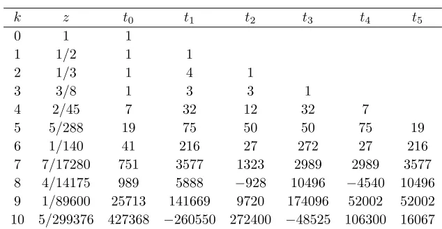
3.1. General closed Newton-Cotes formulae. The closed Newton-Cotes integral rules are given by
Z b
a
f(x)dx≈ z h
k X
i=0
tif(xi) (3.1)
k z t0 t1 t2 t3 t4 t5
0 1 1
1 1/2 1 1
2 1/3 1 4 1
3 3/8 1 3 3 1
4 2/45 7 32 12 32 7
5 5/288 19 75 50 50 75 19
6 1/140 41 216 27 272 27 216
7 7/17280 751 3577 1323 2989 2989 3577
8 4/14175 989 5888 −928 10496 −4540 10496 9 1/89600 25713 141669 9720 174096 52002 52002 10 5/299376 427368 −260550 272400 −48525 106300 16067
Table 1. The coefficient z and its weightsti fori= 1,2, . . . ,5
k z t6 t7 t8 t9 t10
0 1
1 1/2 2 1/3 3 3/8 4 2/45 5 5/288
6 1/140 41
7 7/17280 3577 751
8 4/14175 −928 5888 989
9 1/89600 174096 9720 141669 25713
10 5/299376 106300 −48525 272400 −260550 427368 Table 2. The coefficientz and its weightsti fori= 6,7, . . . ,10
Where
h=b−a
N , xi=a+ih, i= 0,1,2, . . . , N. (3.2) The coefficient z as well as the weightsti are given in Tables 1,2. From tables
1 and 2 it is easy to see that the coefficientstiare symmetric, i.e., we have the
following relation:
ti =tk−i, i= 0,1, . . . ,
k
2. (3.3)
Closed Newton-Cotes differential methods were produced from the integral rules. For Table 1 we have the following differential methods:
k= 1 yn+1−yn=
h
2(fn+1+fn) k= 2 yn+1−yn−1=
h
3(fn−1+ 4fn+fn+1) k= 3 yn+1−yn−2=
3h
8 (fn−2+ 3fn−1+ 3fn+fn+1) k= 4 yn+2−yn−2=
2h
45(7fn−2+ 32fn−1+ 12fn+ 32fn+1+fn+2) k= 5 yn+2−yn−3=
h
140(19fn−3+ 75fn−2+ 50fn−1+ 50fn+ 75fn+1+ 19fn+2) ..
. (3.4)
k= 10 yn+5−yn−5 = 5h
299376(427368fn−260550 (fn+1+fn−1) +272400 (fn+2+fn−2)−48525 (fn+3+fn−3) +106300 (fn+4+fn−4) + 16067 (fn+5+fn−5))
In the present paper we will investigate the casek= 10 and we will produce trigonometrically-fitted differential methods of order 12.
3.2. Trigonometrically-fitted closed Newton-Cotes differential method.
Requiring the differential scheme
yn+5−yn−5=h b0fn+
5
X
i=1
bi(fn+i+fn−i) !
(3.5) to be accurate for the following set of functions (we note that fi = yi0, i =
n−1, n, n+ 1):
{1, x, x2, x3, x4, x5, x6, x7, x8, x9,cos(ωh),sin(ωh)} (3.6) the following set of equations is obtained:
2b1+ 2b2+ 2b3+ 2b4+ 2b5+b0= 10 6b1+ 24b2+ 54b3+ 96b4+ 150b5= 250
2560b4+ 810b3+ 160b2+ 6250b5+ 10b1= 6250
10206b3+ 57344b4+ 14b1+ 218750b5+ 896b2= 156250 118098b3+ 4608b2+ 1179648b4+ 7031250b5+ 18b1= 3906250
−24 sin(v) (cos(v))2+ 2 sin(v) + 32 sin(v) (cos(v))4−2b4v−b0v −8 (cos (v))3b3v−32b5v(cos (v))
5
−16b4v(cos (v)) 4
+ 40 (cos (v))3b5v−10 cos (v)b5v−4 (cos (v)) 2
b2v
+ 16 (cos (v))2b4v+ 6 cos (v)b3v−2b1cos (v)v+ 2b2v= 0
(3.7)
Solving the above system of equations we obtain b0=
1 2268
a0
T b1= 1 4536
a1
T , b2= 1 1134
a2 T ,
b3= 1 9072
a3
T, b4= 1 9072
a4
T, b5= 1 9072
a5 T , where
a0 = 169555vcos5(v) + (426400v−571536 sin(v)) cos4(v) −145625vcos3(v) + (−344200v+ 428652 sin(v)) cos2(v) +60275vcos(v)−35721 sin(v) + 12200v,
a1 = −275350vcos5(v) + (−746875v+ 952560 sin(v)) (cos(v)) 4
+315125v(cos(v))3+ (501250v−714420 sin(v)) (cos(v))2 −64250vcos(v) + 59535 sin(v)−27575v,
a2 = 41675vcos5(v) + (95000v−136080 sin(v)) cos4(v) −21625vcos3(v) + (−95000v+ 102060 sin(v)) cos2(v) +20875vcos(v)−8505 sin(v) + 1600v,
a3 = −116900vcos5(v) + (−325625v+ 408240 sin(v)) cos4(v) +146125vcos3(v) + (203750v−306180 sin(v)) cos2(v) −22000vcos(v)−12925v+ 25515 sin(v),
a4 = 20225vcos5(v)−45360 sin(v) cos4(v) + 56125vcos3(v) + (−95000v+ 34020 sin(v)) cos2(v) + 38625vcos(v) −5800v−2835 sin(v),
a5 = (−20225v+ 9072 sin(v)) cos4(v) + 29225vcos3(v) + (−21450v−6804 sin(v)) cos2(v) + 12500vcos(v) −2885v+ 567 sin(v),
and
T =v(cos(v)−1)5.
For small values ofvthe above formulae are subject to heavy cancellations. In this case the following Taylor series expansions must be used:
b0 =
89035 12474 −
673175 648648v
2+ 19375 2594592v
4+ 395515 264648384v
6
+ 173704325 2534272925184v
8+ 104265059 55754004354048v
10+ 1839935 115700039110656v
12
− 14814979111 8401905440137617408v
14− 19367733685 134430487042201878528v
16+· · · ,
b1 = − 24125 5544 + 3365875 3891888v 2 − 96875 15567552v 4 − 1977575 1587890304v 6 − 868521625 15205637551104v
8− 521325295 334524026124288v
10− 9199675 694200234663936v
12
+ 74074895555 50411432640825704448v
14+ 96838668425 806582922253211271168v
16+· · · ,
b2 =
28375 6237 −
3365875 6810804v
2+ 96875 27243216v
4+ 1977575 2778808032v
6
+ 868521625 26609865714432v
8+ 521325295 585417045717504v
10+ 9199675 1214850410661888v
12
− 74074895555 88220007121444982784v
14− 96838668425
1411520113943119724544v
16+· · · ,
b3 = − 80875 99792 +
3365875 18162144v
2− 96875 72648576v
4− 1977575 7410154752v 6 − 868521625 70959641905152v 8 − 521325295 1561112121913344v 10 − 9199675 3239601095098368v 12 + 74074895555 235253352323853287424v
14+ 96838668425 3764053637181652598784v
16+· · · ,
b4 =
132875 74844 −
3365875 81729648v
2+ 96875 326918592v
4+ 1977575 33345696384v
6
+ 868521625 319318388573184v
8+ 521325295 7025004548610048v
10+ 9199675 14578204927942656v
12
− 74074895555 1058640085457339793408v
14− 96838668425
16938241367317436694528v
16+· · · ,
b5 =
80335 299376+
673175 163459296v
2− 19375 653837184v
4− 395515 66691392768v
6
− 173704325 638636777146368v
8− 104265059 14050009097220096v
10− 1839935 29156409855885312v
12
+ 14814979111 2117280170914679586816v
14+ 19367733685
33876482734634873389056v 16+
· · · .
The local truncation error for the above differential method is given by LT E=− 673175
163459296
yn(13)+ω2yn(11)
h13. (3.8)
4. Closed Newton-Cotes Can be Expressed as Symplectic Integrators
Theorem 4.1. A discrete scheme of the form
b −a
a b
qn+1 pn+1
=
b a
−a b qn
pn
, (4.1)
is symplectic.
Figure 1. Behavior of the coefficientsb0and b1 of the new method.
Figure 2. Behavior of the coefficientsb2and b3 of the new method.
Figure 3. Behavior of the coefficientsb4and b5 of the new method.
Proof. We rewrite (2.3) as
q n+1 pn+1
=
b
−a a b
−1 b a
−a b qn
pn
.
Define
M =
b −a a b
−1
b a −a b
= 1
b2+a2
b2−a2 2ab −2ab b2−a2
and it can easily be verified that
MTJ M =J
thus the matrixM is symplectic. The symplectic structure of the well-known second order differential scheme (SOD) has been proven in [26] by Zhu et al.
yn+i−yn−i= 2ihfn i= 1(1)5 (4.2)
The above methods have been produced by the simplest open Newton-Cotes integral formula. Based on the paper Chiou et al. [2], the closed Newton-Cotes differential schemes will be written as multilayer symplectic structures. If we apply the Newton-Cotes differential formula forn= 5 to the linear Hamiltonian system (1.1) we obtain
qn+5−qn−5=s b0pn+
5
X
i=1
bi(pn+i+pn−i) !
,
pn+5−pn−5=s b0qn+
5
X
i=1
bi(qn+i+qn−i)
! (4.3)
wheres=mh, wheremis defined in (1). From (3.4) we have qn+j−qn−j=2j s pn,
pn+j−pn−j=−2j s qn, j= 1(1)5, orj=
1 2(1)
5 2.
(4.4)
Considering the approximation based on the first formula of (4.1) for (n+ 1)-step gives (taking into account the second formula of (4.1))
qn+i+qn−j =
qn+spn+i−1 2
+qn−spn−i+1 2
= qn+i−1+qn−i+1+s
pn+i−1
2 −pn−i+12
= (2−i2s2)qn. (4.5)
Substituting (4.2)-(4.5) into (3.5) and considering thatbi=b5−i,i= 0(1)4, we
have
qn+5−qn−5 = s
h
b5(pn−5+pn+5) + b4(2−42s2) +b3(2−32s2)
+b2(2−22s2) +b1(2−s2) +b0pn i
, (4.6)
pn+5−pn−5 = s
h
b5(qn−5+qn+5) + b4(2−42s2) +b3(2−32s2)
+b2(2−22s2) +b1(2−s2) +b0
qn i
,
and with (3.6) we have qn+5−qn−5 = s
h
b5(pn−5+pn+5) + b4(2−42s2) +b3(2−32s2) +b2(2−22s2) +b1(2−s2) +b0
qn+5−qn−5 10s
i
,
pn+5−pn−5 = s
h
b5(qn−5+qn+5) + b4(2−42s2) +b3(2−32s2)
+b2(2−22s2) +b1(2−s2) +b0
pn+5−pn−5 10s
i
,
which gives
(qn+5−qn−5).A=s b0(pn+5+pn−5),
(pn+5−pn−5).B=s b0(qn+5+qn−5).
where
A= 1−b4(2−4
2s2) +b3(2−32s2) +b2(2−22s2) +b1(2−s2) +b 0
10 ,
and
B= 1−b4(2−4
2s2) +b3(2−32s2) +b2(2−22s2) +b1(2−s2) +b 0
10 .
The above formula in matrix form can be written as
T(s) −s b5 s b5 T(s)
qn+5 pn+5
=
T(s) s b5 −s b5 T(s)
qn−5 pn−5
where
T(s) = 1−b4(2−4
2s2) +b
3(2−32s2) +b2(2−22s2) +b1(2−s2) +b0
10 (4.7)
which is a discrete scheme of the form (3.3) and hence it is symplectic. 5. Error Analysis for the Radial Schr¨odinger Equation In this section, we will investigate theoretically the methods constructed in [21, 22, 23, 24, 25] and in this paper. The scope of this investigation is to find a quantitative estimation for the extent of the accuracy gain to be expected from the exponentially-fitted versions.
Definition 5.1. A method is called classical if it has constant coefficients. Remark 5.2. A trigonometrically-fitted method is not a classical one because it has coefficients which are dependent on the quantityv=ω h, wherewis the frequency of the problem andhis the step length of the integration.
Consider the radial Schr¨odinger equation y00(x) =
l(l+ 1)
x2 +V(x)−k 2
y(x) =f(x)y(x). (5.1) wheref(x) =U(x)−k2andU(x) =l(l+ 1)/x2+V(x). We writef(x) in (5.1) in the form
f(x) =g(x) +d, (5.2)
where g(x) =U(x)−Uc =g, where Uc is the constant approximation of the
potential andG=v2=U
c−E.
So, g(x) depends on the potential and the constant approximation of the potential whiledshows the energy dependence. We will compare the following methods:
•The classical fourth order closed Newton-Cotes formulae (Method I). •The classical sixth order closed Newton-Cotes formulae (Method II). •The classical eighth order closed Newton-Cotes formulae (Method III). •The closed Newton-Cotes formulae developed in [21] (Method IV). •The closed Newton-Cotes formulae developed in [19] (Method V). •The closed Newton-Cotes formulae developed in [23] (Method VI). •The classical tenth order closed Newton-Cotes formulae (Method VII) •The closed Newton-Cotes formulae developed in the paragraph 3.2, in [22] (Method VIII).
•The closed Newton-Cotes formulae developed in the paragraph 3.3 in [22] (Method IX).
•The closed Newton-Cotes formulae developed in this paper (Method X). We now present the formulae of the local truncation error (LTE) for the above methods.
For the Method I is equal to:
LT EM I =−
h5 90y
(5)
n .
For the Method II is equal to:
LT EM II =−
8h5 945y
(7)
n .
For the Method III is equal to:
LT EM III =−
9h9 1400y
(9)
n .
For the Method IV is equal to:
LT EM IV =−
8h9 945(y
(7)
n +v
2y(5)
n ).
For the Method V is equal to:
LT EM V =−
h5 90(y
(5)
n +v2yn(3)).
For the Method VI is equal to:
LT EM V I =−
9h5 1400(y
(9)
n + 3v
2y(7)
n + 3v
4y(5)
n +v
6y(3)
n ).
For the Method VII is equal to:
LT EM V II=−
2368 467775y (11) n h 11 .
For the Method VIII is equal to:
LT EM V III=−
2368 467775
yn(11)+ 2ν2yn(9)+ν4yn(7)h11. For the Method IX is equal to:
LT EM IX =−
2368 467775
yn(11)+ 5ν2y(9)n + 4ν4yn(7)h11. For the new Method (Method X) is equal to:
LT EM X =−
673175 163459296
y(13)n +v2yn(11)h13.
We express, now, the derivativesy(2),y(4),. . .andy(13) in terms of Eq. (5.1), ie.
yn(2) = f(x).y(x), yn(3) =
d
dxg(x)
y(x) + (g(x) +d)d dxy(x) yn(5) =
d3
dx3g(x)
y(x) + 3
d2
dx2g(x)
d
dxy(x), +3
d
dxg(x)
d2
dx2y(x) + (g(x) +d) d3
dx3y(x), (5.3) and etc. We note thatg(n)=U(n)(x) for then-th order derivative with respect to x. Introducing the expressions obtained in (5.3) into the Local Truncation Error of the methods mentioned above, we obtain the expressions (as polyno-mials ofd) for local truncation error of the methods. The leading terms (ind) of the above expressions are given by:
For the Method I is equal to:
LT EM I=h5d2
−1 90
d dxy(x)
.
For the Method II is equal to:
LT EM II =h7d3
− 8 945
d dxy(x)
.
For the Method III is equal to:
LT EM III =h9d4
− 9 1400
d dxy(x)
.
For the Method IV is equal to:
LT EM IV =−
8 945
g(x) d
dxy(x) + 5
d dxg(x)
y(x)
h9d2.
For the Method V is equal to:
LT EM V =−
1 90
d
dxy(x)
g(x) + 3
d
dxg(x)
y(x)
h9d.
For the Method VI is equal to:
LT EM V I = −
9 700 3
d
dxg(x)
y(x)g(x) + 8
d3
dx3g(x)
y(x)
+2
d2
dx2g(x)
d
dxy(x)
!
h9d2.
For the Method VII is equal to:
LT EM V II=h11d5
− 2368 467775
d dxy(x)
.
For the Method VIII is equal to:
LT EM V III =h11d4
− 4736 467775y(x)
d dxg(x)
.
For the Method IX is equal to:
LT EM IX =
2368 155925h
11d4
19
3
d
dxg(x)
y(x) +
d
dxy(x)
g(x)
.
For the Method X is equal to:
LT EM X =−
673175 163459296
g(x) d
dxy(x) + 11
d
dxg(x)
y(x)
h13d5.
From the above equations we have the following theorem:
Theorem 5.3. For the Closed Newton-Cotes formulae studied in this paper we have:
• Fourth Algebraic Order Methods
In the fourth algebraic order method MI the error increases as the second power of d, while in the fourth algebraic order method MV the the error increases as the first power ofd. So, for the numerical solution of the time independent radial Schr¨odinger equation the Method MV is more accurate, especially for large values ofd.
• Sixth Algebraic Order Methods
In the sixth algebraic order method MII the error increases as the third power ofd, while in the sixth algebraic order method MIV the the error increases as the second power ofd. So, for the numerical solution of the time independent radial Schr¨odinger equation the Method MIV is more accurate, especially for large values ofd.
• Eighth Algebraic Order Methods
In the eighth algebraic order method MIII the error increases as the fourth power of d, while in the eighth algebraic order method MVI the the error increases as the second power ofd. So, for the numerical so-lution of the time independent radial Schr¨odinger equation new Method MVI is more accurate, especially for large values ofd.
• Tenth Algebraic Order Methods
In the tenth algebraic order method MVII the error increases as the fifth power ofd, while in the tenth algebraic order methods MVIII and MIX the the error increases as the fourth power ofd. The coefficient of the fourth power ofd in the Method MVIII is much lower than the coefficient of the fourth power of d in the Method MIX. So, for the numerical solution of the time independent radial Schr¨odinger equation new Methods MVIII is the most accurate one, especially for large values of d.
• Twelfth Algebraic Order Methods
In the twelfth algebraic order method MX the error increases as the fifth power ofd. So, for the numerical solution of the time independent radial Schr¨odinger equation new Methods MX is the most accurate one, especially for large values ofd.
6. Numerical Results
In this section we present some numerical results to illustrate the per-formance of our new methods. Consider the numerical integration of the Schr¨odinger equation:
y00(x) =
l(l+ 1)
x2 +V(x)−k 2
y(x), (6.1)
using the well-known Woods-Saxon potential which is given by V(x) =Vw=
u0 1 +z−
u0z
a(1 +z)2, (6.2)
with z = exp[(x−R0)/a], u0 = −50, a = 0.6, and R0 = 7.0. In Fig. 2, we give a graph of this potential. In the case of negative eigenenergies (i.e. whenE∈[−50,0]) we have the well-known bound-states problem while in the case of positive eigenenergies (i.e. whenE∈(0,1000]) we have the well-known resonance problem. Many problems in chemistry, physics, physical chemistry, chemical physics, electronics etc., are expressed by Eq. (6.1).
6.1. Resonance problem. In the case of positive energies, E =k2, the po-tential dies away faster than the term l(lx+1)2 and the Schr¨odinger equation
Figure 4. The Woods - Saxon potential. effectively reduces to
y00(x) =
k2−l(l+ 1) x2
y(x), (6.3)
forxgreater than some valueX. The last equation has two linearly independent solutions kxjl(kx) and kxnl(kx), where jl(kx) and nl(kx) are the spherical
Bessel and Neumann functions respectively. Thus the solution of Eq. (6.1) has When (x→ ∞) the solution takes the asymptotic form
y(x) ≈ A k x jl(k x)−B k x nl(k x)
≈ D[sin(k x−πl/2) + tan(δl) cos(kx−πl/2)],
whereδlis calledscattering phase shiftthat may be calculated from the formula
tan(δl) =
y(xi)S(xi+1)−y(xi+1)S(xi)
y(xi+1)C(xi)−y(xi,)C(xi+1)
(6.4) for x1 and x2 distinct points in the asymptotic region (we choose x1 as the right-hand end point of the interval of integration andx2=x1−h)withS(x) = kxjl(kx) and C(x) = −kxnl(kx). Since the problem is treated as an
initial-value problem, we needy0before starting a eight-step method. From the initial condition we obtain y0. With these starting values we evaluate at x1 of the asymptotic region the phase shiftδl from the above relation.
6.1.1. The woods-saxon potential. As a test for the accuracy of our methods we consider the numerical integration of the Schr¨odinger equation (6.1) withl= 0 in the well-known case where the potentialV(r) is the Woods-Saxon one (6.2). One can investigate the problem considered here, following two procedures. The first procedure consists of finding the phase shiftδ(E) =δl forE ∈[1,1000].
The second procedure consists of finding those E, forE ∈[1,1000], at which δ equalsπ/2. In our case we follow the first procedure i.e. we try to find the phase shifts for given energies. The obtained phase shift is then compared to the analytic value of π/2. The above problem is the so-called resonance problem when the positive eigenenergies lie under the potential barrier.We solve this problem, using the technique fully described in [1]. The boundary conditions for this problem are:
y(0) = 0, y(x)≈cos(√Ex), for large x. (6.5) The domain of numerical integration is [0,15].
For comparison purposes in our numerical illustration we use the following methods:
• The well known Numerov’s method (which is indicated as Method A). • The exponentially-fitted method of Raptis and Allison [11] (which is
indicated as Method B).
• The P-stable exponentially-fitted Method developed by Kalogiratou and Simos [6] (which is indicated as Method C)
• The four-step method developed by Henrici [3] (which is indicated as Method D).
• The Newton-Cotes trigonometrically-fitted formula developed in [20] (which is indicated as Method E).
• The Newton-Cotes trigonometrically-fitted formula developed in [23] (which is indicated as Method F).
• The Newton-Cotes trigonometrically-fitted formula developed in [24] (which is indicated as Method G).
• The Newton-Cotes exponentially-fitted method developed in [22] (which is indicated as Method H).
• The Newton-Cotes trigonometrically-fitted method developed in [22] (which is indicated as Method I).
• The new proposed trigonometrically-fitted method (which is indicated as Method J).
The numerical results obtained for the six methods, with several number of function evaluations (NFE), were compared with the analytic solution of the Woods-Saxon potential resonance problem, rounded to six decimal places. Fig-ure , show the errors Err = −log10|Ecalculated −Eanalytical| of the highest
eigenenergy E3 = 989.701916 for several values of NFE, where NFE are the Number of Function Evaluations.
7. Conclusions
In this paper a new high order closed Newton-Cotes differential method for the numerical solution of the Schr¨odinger type equations is introduced.
From the numerical results we have the following remarks:
Figure 5. Error Errmax for several values ofnfor the eigen-valueE1= 989.701916. The nonexistence of a value of Errmax indicates that for this value ofn, Errmax is positive
• The Numerovs method and the exponentially-fitted method of Raptis and Allison [11] have better behavior than the P-stable exponentially-fitted method developed by Kalogiratou and Simos [6].
• The exponentially-fitted method of Raptis and Allison [11] is more efficient than the well known Numerov method.
• The four-step method developed by Henrici [3] has better behavior than all the previous mentioned methods. The Newton-Cotes trigonometrically-fitted formula developed in [20] has better behavior than all the above methods.
• The Newton-Cotes trigonometrically-fitted formula developed in [22] is more efficient than all the above methods. The behavior of the Newton-Cotes trigonometrically-fitted formula developed in [24] is bet-ter than all the above methods.
• The new proposed trigonometrically-fitted method is more efficient than all the above methods.
• Finally, the new developed exponentially-fitted method is the most efficient one.
Remark 7.1. As the theoretical and numerical results show us, for the de-velopment of numerical methods for the approximate solution of the radial Schr¨odinger equation, the exponentially-fitted methodology gives much more efficient methods than the trigonometrically-fitted methodology.
Acknowledgments
The authors wish to thank the anonymous referees for their careful reading of the manuscript and their fruitful comments and suggestions.
References
1. Z.A. Anastassi, T.E., Simos, Trigonometrically-fitted Runge-Kutta methods for the
nu-merical solution of the Schr¨odinger equation,Journal of Mathematical Chemistry,37(3),
(2005), 281-293.
2. J. C. Chiou, S. D. Wu, Open Newton-Cotes differential methods as multilayer symplectic
integrators,Journal of Chemical Physics,107, (1997), 6894-6897.
3. P. Henrici,Discrete Variable Methods in Ordinary Differential Equations, Wiley, New
York, 1962.
4. M.K. Jain, R.K. Jain, U.A. Krishnaiah, Obrechkoff methods for periodic initial value
problems of second order differential equations,Journal of Mathematical Physics,15,
(1981), 239-250.
5. B. Jazbi , M. Moini, Application of Hes homotopy perturbation method for Schr¨odinger
equation,Iranian Journal of Mathematical Sciences and Informatics,3(2), (2008), 13-19.
6. Z. Kalogiratou, T.E. Simos, A P-stable exponentially-fitted method for the numerical
integration of the Schr¨odinger equation,Applied Mathematics and Computations,112,
(2000), 99-112.
7. J.D. Lambert, Numerical methods for ordinary differential systems, The initial value
problem, John Wiley and Sons, 1991.
8. J.D. Lambert, I.A. Watson, Symmetric multistep methods for periodic initial value
prob-lems,Journal of the Institute of Mathematics and its Applications,18, (1976), 189-202.
9. P. Mokhtary, S.M. Hosseini, Some implementation aspects of the general linear
meth-ods withinherent Runge-Kutta stability,Iranian Journal of Mathematical Sciences and
Informatics,3(1), (2008), 63-76.
10. G. D. Quinlan, S. Tremaine, Symmetric multistep methods for the numerical integration
of planetary orbits, The Astro,The Astronomical Journal,100(5), (1990), 1694-1700.
11. A. D. Raptis, A. C. Allison, Exponential-fitting methods for the numerical solution of
the Schr¨odinger equation, Journal of Computer Physics Communications,14, (1978),
1-5.
12. A. Shokri, An explicit trigonometrically fitted ten-step method with phase-lag of order
infinity for the numerical solution of radial Schr¨odinger equation,Applied and
Compu-tational Mathematics,14(1), (2015), 63-74.
13. A. Shokri, The symmetric two-step P-stable nonlinear predictor-corrector methods for
the numerical solution of second order initial value problems, Bulletin of the Iranian
Mathematical Society,41(1), (2015), 191-205.
14. A. Shokri, A.A. Shokri, S. Mostafavi, H. Saadat, Trigonometrically fitted two-step
Obrechkoff methods for the numerical solution of periodic initial value problems,
Ira-nian Journal of Mathematical Chemistry,6(2), (2015), 145-161.
15. A. Shokri, H. Saadat, Trigonometrically fitted high-order predictor-corrector method
with phase-lag of order infinity for the numerical solution of radial Schr¨odinger equation,
Journal of Mathematical Chemistry,52(7), (2014), 1870-1894.
16. A. Shokri, H. Saadat, High phase-lag order trigonometrically fitted two-step Obrechkoff
methods for the numerical solution of periodic initial value problems,Numerical
Algo-rithms,68, (2015), 337-354.
17. A. Shokri, A. A. Shokri, The new class of implicit L-stable hybrid Obrechkoff method for
the numerical solution of first order initial value problems,Journal of Computer Physics
Communications,184, (2013), 529-531.
18. T. E. Simos, Accurately closed Newton-Cotes trigonometrically-fitted formulae for the
numerical solution of the Schr¨odinger equation,International Journal of Modern Physics
C,24(3), (2013).
19. T. E. Simos, Closed Newton-Cotes trigonometrically-fitted formulae for long-time
in-tegration of orbital problems, Revista Mexicana de Astronomia y Astrofysica, 42(2),
(2006), 167-177.
20. T. E. Simos, Closed Newton-Cotes trigonometrically-fitted formulae of high-order for
long-time integration of orbital problems,Applied Mathematical Letters,22(10), (2009),
1616-1621.
21. T. E. Simos, Closed Newton-Cotes trigonometrically-fitted formulae for long-time
inte-gration,International Journal of Modern Physics C,14(8), (2003), 1061-1074.
22. T. E. Simos, High order closed Newton-Cotes exponentially and trigonometrically fit-ted formulae as multilayer symplectic integrators and their application to the radial
Schr¨odinger equation,Journal of Mathematical Chemistry,50(5), (2012), 1224-1261.
23. T. E. Simos, High-order closed Newton-Cotes trigonometrically-fitted formulae for
long-time integration of orbital problems, Journal of Computer Physics Communications,
178(3), (2008), 199-207.
24. T. E. Simos, High order closed Newton-Cotes trigonometrically-fitted formulae for the
numerical solution of the Schr¨odinger equation,Applied Mathematics and Computation,
209 (1), (2009), 137-151.
25. T. E. Simos, New closed Newton-Cotes type formulae as multilayer symplectic
integra-tors,Journal of Chemical Physics,133(10), (2010), 104-108.
26. W. Zhu, X. Zhao, Y. Tang, Numerical methods with a high order of accuracy in the
quantum system,Journal of Chemical Physics,104, (1996) 2275-2286.