Numerical Solution of Second Kind Volterra and Fredholm Integral Equations Based on a Direct Method Via Triangular Functions

Vol. 11, No. 2, 2019 Article ID IJIM-001062, 9 pages Research Article

Numerical Solution of Second Kind Volterra and Fredholm Integral

Equations Based on a Direct Method Via Triangular Functions

S. Hatamzadeh-Varmazyar ∗†, Z. Masouri ‡

Received Date: 2017-04-27 Revised Date: 2018-07-31 Accepted Date: 2018-12-02

————————————————————————————————–

Abstract

A numerical method for solving linear Volterra and Fredholm integral equations of the second kind is formulated. Based on a special representation of vector forms of triangular functions (TFs) and the related operational matrix of integration, the integral equation reduces to a linear system of algebraic equations. The generation of this system needs no integration, so all calculations can easily be implemented. Numerical results for some examples show that the method has a good accuracy.

Keywords: Integral equations of the second kind; Direct method; Vector forms; Triangular functions; Approximate solution.

—————————————————————————————————–

1

Introduction

N

integral and integro-differential equations, because a great number of problems in physi-cal science and engineering are modeled by such equations [6,5,2,15,11,13,16,17,9,3,10,4,18]. This paper uses the TFs as a set of orthogonal basis functions for formulation of a direct method for solving both Volterra and Fredholm integral equations of the second kind. For this purpose, we review the TFs and a special representation of their vector forms as well as the related op-erational matrix of integration. Then, the direct method is formulated for numerical solution of the second kind integral equations. Finally, some examples are solved by the method. The obtained results are compared with those of other methods

∗_{Corresponding author. [email protected].} †_{Department of Electrical Engineering, Islamshahr} Branch, Islamic Azad University, Tehran, Iran.

‡_{Department of Mathematics, Islamshahr Branch,} Is-lamic Azad University, Tehran, Iran.

to illustrate the efficiency and accuracy of the di-rect method for solving the mentioned integral equations.

2

Review

of

triangular

func-tions

2.1 Definition

Two m-sets of TFs are defined over the interval [0, T) as [7,6]

T1i(t) =

{

1−t−_hih, ih≤t <(i+ 1)h,

0, otherwise,

T2i(t) =

{

t−ih

h , ih≤t <(i+ 1)h,

0, otherwise,

(2.1)

where i= 0,1, . . . , m−1, with a positive integer value form. Also, consider h=T /m, andT1i as

the ith left-handed TF and T2i as the ith

right-handed TF.

In this paper, it is assumed thatT = 1, so TFs are defined over [0,1), andh= 1/m.

From the definition of TFs, it is clear that they are disjoint, orthogonal, and complete [7]. There-fore, we can write

∫ 1

0

T1i(t)T1j(t)dt=

∫ 1

0

T2i(t)T2j(t)dt

= {

h

3, i=j, 0, i̸=j.

(2.2)

Also,

φi(t) =T1i(t) +T2i(t), i= 0,1, . . . , m−1,

(2.3) whereφi(t) is the ith BPF defined as

φi(t) = {

1, ih⩽t <(i+ 1)h,

0, otherwise, (2.4)

wherei= 0,1, ..., m−1.

2.2 Vector forms

Consider the firstmterms of left-handed TFs and the first m terms of right-handed TFs and write them concisely as m-vectors:

T1(t) = [T10(t), T11(t), ..., T1m−1(t)]T,

T2(t) = [T20(t), T21(t), ..., T2m−1(t)]T,

(2.5)

where T1(t) and T2(t) are called left-handed triangular functions (LHTF) vector and right-handed triangular functions (RHTF) vector, re-spectively.

The following properties of the product of two TFs vectors may be obtained [6]:

T1(t)T1T(t)

≃     

T10(t) 0 . . . 0 0 T11(t) . . . 0

..

. ... . .. ... 0 0 . . . T1m−1(t)

    ,

T2(t)T2T(t)

≃     

T20(t) 0 . . . 0 0 T21(t) . . . 0

..

. ... . .. ... 0 0 . . . T2m−1(t)

    ,

(2.6)

and

T1(t)T2T(t)≃0,

T2(t)T1T(t)≃0,

(2.7)

where 0is the zero m×m matrix. Also,

∫ 1

0

T1(t)T1T(t)dt= ∫ 1

0

T2(t)T2T(t)dt

≃ h 3I,

∫ 1

0

T1(t)T2T(t)dt= ∫ 1

0

T2(t)T1T(t)dt

≃ h 6I,

(2.8)

in which I is m×m identity matrix.

2.3 TFs expansion

The expansion of a functionf(t) over [0,1) with respect to TFs, may be compactly written as

f(t)≃

m∑−1

i=0

ciT1i(t) + m∑−1

i=0

diT2i(t)

=cTT1(t) +dTT2(t),

(2.9)

where we may putci=f(ih) anddi=f((i+ 1)h)

fori= 0,1, . . . , m−1. So, approximating a known

function by TFs needs no integration to evaluate the coefficients.

2.4 Operational matrix of integration

Expressing ∫₀sT1(τ)dτ and ∫₀sT2(τ)dτ in terms of TFs follows [7]:

∫ s

0

T1(τ)dτ ≃P1T1(s) +P2T2(s),

∫ s

0

T2(τ)dτ ≃P1T1(s) +P2T2(s),

(2.10)

whereP1m×m andP2m×m are called operational

repre-sented as follows:

P1 = h 2       

0 1 1 . . . 1 0 0 1 . . . 1 0 0 0 . . . 1

..

. ... ... . .. ... 0 0 0 . . . 0

       ,

P2 = h 2       

1 1 1 . . . 1 0 1 1 . . . 1 0 0 1 . . . 1

..

. ... ... . .. ... 0 0 0 . . . 1

       . (2.11)

So, the integral of any function f(t) can be ap-proximated as

∫ s

0

f(τ)dτ ≃

∫ s

0 [

cTT1(τ) +dTT2(τ)]dτ

≃(c+d)TP1T1(s) + (c+d)TP2T2(s).

(2.12)

3

A special representation of

TFs vector forms and other

properties

In this section, we review a special representa-tion of TFs vector forms that has originally been introduced in [6].

3.1 Definition and expansion

LetT(t) be a 2m-vector defined as [6]

T(t) =  T1(t)

T2(t) 

, 0⩽t <1 (3.13)

whereT1(t) andT2(t) have been defined in (2.5). Now, the expansion of f(t) with respect to TFs can be written as

f(t)≃F1TT1(t) +F2TT2(t)

=FTT(t)

=TT(t)F,

(3.14)

whereF1 andF2 are TFs coefficients withF1i = f(ih) andF2i=f((i+ 1)h), for i= 0,1, . . . , m−

1. Also, 2m-vector F is defined as

F =  F1

F2 

. (3.15)

Now, assume that k(s, t) is a function of two variables. It can be expanded with respect to TFs as follows:

k(s, t)≃TT(s) K T(t), (3.16)

where T(s) and T(t) are 2m1- and 2m2 -dimensional TFs respectively, and K is a 2m1× 2m2 TFs coefficient matrix. For convenience, we putm1=m2 =m. So, matrixK can be written as

K= 

(K11)m×m (K12)m×m (K21)m×m (K22)m×m



, (3.17)

where K11, K12, K21, and K22 can be com-puted by sampling of function k(s, t) at pointssi

and ti such that si =ti =ih, for i= 0,1, . . . , m. Therefore,

(K11)i,j =k(si, tj), i= 0,1, . . . , m−1, j= 0,1, . . . , m−1,

(K12)i,j =k(si, tj), i= 0,1, . . . , m−1,

j= 1,2, . . . , m,

(K21)i,j =k(si, tj), i= 1,2, . . . , m,

j= 0,1, . . . , m−1,

(K22)i,j =k(si, tj), i= 1,2, . . . , m,

j= 1,2, . . . , m.

(3.18)

3.2 Product properties

Let X be a 2m-vector which can be written as

XT = (X1T X2T) such that X1 and X2 are

m-vectors. Now, it can be concluded from Eqs. (2.6) and (2.7) that [6]:

T(t)TT(t)X

= (

T1(t) T2(t)

) (

T1T(t) T2T(t)) (X1

X2 )

≃ 

diag(T1(t)) 0m×m

0m×m diag(T2(t))

 

 X1

X2  

=diag(T(t)) X

=diag(X) T(t).

(3.19)

Therefore,

T(t)TT(t)X ≃X˜T(t), (3.20)

Now, let B be a 2m×2m matrix as:

B = 

(B11)m×m (B12)m×m (B21)m×m (B22)m×m



. (3.21)

So, it can be similarly concluded from Eqs. (2.6) and (2.7) that:

TT(t)BT(t)

=(T1T(t) T2T(t)) (B11 B12

B21 B22 ) (

T1(t) T2(t)

)

≃T1T(t)B11 T1(t) +T2T(t)B22 T2(t) ≃_Bˆ₁₁T _{T1(t) + ˆB22}T _T2(t),

(3.22)

where ˆB11 and ˆB22 arem-vectors with elements equal to the diagonal entries of matricesB11 and

B22, respectively. Therefore,

TT(t)BT(t)≃BˆTT(t), (3.23)

in which ˆB is a 2m-vector with elements equal to the diagonal entries of matrix B. Also, it is immediately concluded from Eqs. (2.8):

∫ 1

0

T(t)TT(t) dt

= ∫ 1

0 (

T1(t) T2(t)

) (

T1T(t) T2T(t))dt

= ∫ 1

0 

T1(t)T1

T_{(t) T1(t)T2}T_(t)

T2(t)T1T(t) T2(t)T2T(t)  dt ≃   h

3Im×m

h

6Im×m

h

6Im×m

h

3Im×m  . (3.24) Therefore, ∫ 1 0

T(t)TT(t) dt≃D, (3.25)

whereD is the following 2m×2m matrix:

D= h 3           

1 0 . . . 0 1/2 0 . . . 0 0 1 . . . 0 0 1/2 . . . 0 ..

. ... . .. ... ... ... . .. ... 0 0 . . . 1 0 0 . . . 1/2 1/2 0 . . . 0 1 0 . . . 0

0 1/2 . . . 0 0 1 . . . 0 ..

. ... . .. ... ... ... . .. ... 0 0 . . . 1/2 0 0 . . . 1

           . (3.26)

3.3 Operational matrix

Expressing∫₀sT(τ)dτ in terms ofT(s), and from Eqs. (2.10), we can write [6]

∫ s

0

T(τ)dτ = ∫ s

0 (

T1(τ) T2(τ) )

dτ

≃ 

P1T1(s) +P2T2(s)

P1T1(s) +P2T2(s)  

= 

P1 P2

P1 P2  

 T1(s)

T2(s)  , (3.27) so, _∫ s 0

T(τ)dτ ≃PT(s), (3.28)

where P2m×2m, operational matrix of T(s), is:

P = 

P1 P2

P1 P2 

, (3.29)

where P1 and P2 are given by (2.11).

Now, the integral of any function f(t) can be approximated as

∫ s

0

f(τ)dτ ≃

∫ s

0

FTT(τ)dτ

≃FTPT(s).

(3.30)

4

Direct method for solving

lin-ear second kind integral

equa-tions

Here, by using the results obtained in the pre-vious sections as to the TFs, a numerical direct method for solving second kind integral equations is formulated. The formulation is given for both Volterra and Fredholm integral equations.

4.1 Volterra integral equation

Let us consider the following linear Volterra inte-gral equation of the second kind:

x(s) +λ

∫ s

0

k(s, t)x(t)t=y(s), 0⩽s <1,

(4.31) where the parameter λ and the functions y(s) and k(s, t) are known but x(s) is not. Moreover,

Approximating the functions x(s), y(s), and

k(s, t) with respect to TFs, using (3.14) and (3.16), gives

x(s)≃XTT(s) =TT(s)X,

y(s)≃YTT(s) =TT(s)Y,

k(s, t)≃TT(s)KT(t),

(4.32)

where 2m-vectorsXandY, and 2m×2mmatrix

K are TFs coefficients of x(s), y(s), and k(s, t), respectively. Note that in (4.32), X is the un-known vector and should be computed.

Substituting (4.32) into (4.31) gives

YTT(s)≃XTT(s)

+λ

∫ s

0

TT(s)KT(t)TT(t)Xt. (4.33)

Using Eq. (3.20) follows

YTT(s)≃XTT(s) +λTT(s)K

∫ s

0 ˜

XT(t)t

≃XTT(s) +λTT(s)KX˜

∫ s

0

T(t)t.

(4.34)

Using operational matrixP, in Eq. (3.28), results in

YTT(s)≃XTT(s) +λTT(s)KXP˜ T(s), (4.35)

in which λKXP˜ is a 2m×2m matrix. Using Eq. (3.23) follows

TT(s)λKXP˜ T(s)≃XˆTT(s), (4.36)

where ˆX is a 2m-vector with components equal to the diagonal entries of matrix λKXP˜ .

Now, combining (4.35) and (4.36) and replac-ing≃ with =, we obtain

X+ ˆX=Y. (4.37)

Equation (4.37) is a linear system of 2m

algebraic equations for the 2m unknowns

X10, X11, . . . , X1m−1, X20, X21, . . . , X2m−1, components of XT = (X1T X2T). Hence, an approximate solution x(s) ≃ XTT(s), or

x(s)≃X1TT1(s) +X2TT2(s) can be computed for integral equation (4.31) without using any projection method.

4.2 Fredholm integral equation

Let us consider the following linear Fredholm in-tegral equation of the second kind:

x(s) +λ

∫ 1

0

k(s, t)x(t)t=y(s), 0⩽s <1,

(4.38) where the parameter λ and the functions y(s) and k(s, t) are known and x(s) is the unknown function to be determined. Moreover, k(s, t) ∈

L2([0,1)×[0,1)) and y(s)∈ L2([0,1)). Without loss of generality, it is supposed that the interval of integration in Eq. (4.38) is [0,1), since any fi-nite interval [a, b) can be transformed to interval [0,1) by linear maps [8].

Similar to the direct method for Volterra inte-gral equation, substituting (4.32) into (4.38) fol-lows

YTT(s)≃XTT(s)

+λTT(s)K

∫ 1

0

T(t)TT(t)Xt. (4.39)

Using Eq. (3.25) gives

YTT(s)≃XTT(s) + (λKDX)TT(s). (4.40)

Now, replacing ≃with = results in

(I+λKD)X=Y. (4.41)

Equation (4.41) is a linear system of algebraic equations. So, an approximate solution x(s) ≃

XTT(s) = X1TT1(s) +X2TT2(s), is obtained for Eq. (4.38). Note that, this approach does not use any projection method such as collocation, Galerkin, etc.

5

Test examples

Here, the given direct method is applied to solve some examples. The numerical results obtained by the method are compared with both the exact solution and those obtained by some other meth-ods such as block-pulse functions (BPFs) method, rationalized Haar wavelet method [19], Legen-dre wavelet method [21], Adomian decomposition method [1], and expansion-iterative method [14].

5.1 Numerical results

Example 5.1 Consider the following Fredholm integral equation [19,8]:

x(s)− ∫ 1

0

estx(t)t=es−e

s+1₋₁

Table 1: Numerical results for Example5.1

Exact Solution Direct Direct BPFs Rationalized Haar s method method method wavelet method [19]

(m= 16) (m= 32) (m= 32) (k= 32)

0 1 0.997376 0.999344 1.016236 1.01642

0.1 1.105171 1.102930 1.104568 1.116091 1.11627

0.2 1.221403 1.218903 1.220824 1.225752 1.22593

0.3 1.349859 1.347264 1.349264 1.346191 1.34637

0.4 1.491825 1.489399 1.491158 1.478465 1.47864

0.5 1.648721 1.645485 1.647912 1.675268 1.62391

0.6 1.822119 1.819638 1.821429 1.839883 1.84004

0.7 2.013753 2.010978 2.013136 2.020674 2.02082

0.8 2.225541 2.222754 2.224933 2.219234 2.21936

0.9 2.459603 2.457250 2.458916 2.437307 2.43742

Table 2: Numerical results for Example5.2

.

Exact Solution Direct Direct BPFs Legendre

s method method method wavelet

(m= 16) (m= 32) (m= 32) method [21]

0 1 0.999374 0.999844 1.031832 1.012990

0.1 1.221403 1.222909 1.221598 1.244627 —

0.2 1.491825 1.492803 1.492294 1.501307 1.487708

0.3 1.822119 1.823200 1.822684 1.810922 —

0.4 2.225541 2.228355 2.225880 2.184388 2.230965

0.5 2.718282 2.716581 2.717857 2.804810 —

0.6 3.320117 3.324211 3.320648 3.383247 3.307555

0.7 4.055200 4.057859 4.056475 4.080975 —

0.8 4.953032 4.955970 4.954570 4.922595 4.962956

0.9 6.049647 6.057297 6.050568 5.937783 —

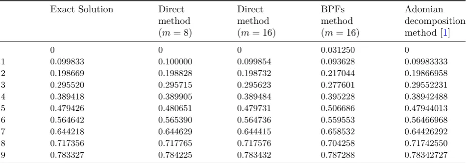
Table 3: Numerical results for Example5.3

.

Exact Solution Direct Direct BPFs Adomian

s method method method decomposition

(m= 8) (m= 16) (m= 16) method [1]

0 0 0 0 0.031250 0

0.1 0.099833 0.100000 0.099854 0.093628 0.09983333

0.2 0.198669 0.198828 0.198732 0.217044 0.19866958

0.3 0.295520 0.295715 0.295623 0.277601 0.29552231

0.4 0.389418 0.389905 0.389484 0.395228 0.38942488

0.5 0.479426 0.480651 0.479731 0.506686 0.47944013

0.6 0.564642 0.565390 0.564736 0.559553 0.56466968

0.7 0.644218 0.644629 0.644415 0.658532 0.64426292

0.8 0.717356 0.717765 0.717576 0.704258 0.71742550

0.9 0.783327 0.784225 0.783432 0.787288 0.78342727

with exact solution x(s) =es. The numerical re-sults are shown in Table 1.

Example 5.2 For the following Fredholm

inte-gral equation of the second kind [21, 20]:

x(s) + ∫ 1

0 1 3e

2s−5₃t_x(t)t=e2s+1_{3, (5.43)}

Table 4: Numerical results for Example5.4

.

Exact Direct Direct Expansion-iterative s solution method method method [14]

(m= 16) (m= 32) (m= 32)

0 0 0 0 0.015625

0.1 0.100000 0.099998 0.100000 0.109375

0.2 0.200000 0.199986 0.199997 0.203125

0.3 0.300000 0.299955 0.299989 0.296875

0.4 0.400000 0.399895 0.399974 0.390625

0.5 0.500000 0.499801 0.499950 0.515625

0.6 0.600000 0.599663 0.599916 0.609375

0.7 0.700000 0.699488 0.699872 0.703125

0.8 0.800000 0.799282 0.799820 0.796875

0.9 0.900000 0.899065 0.899766 0.890625

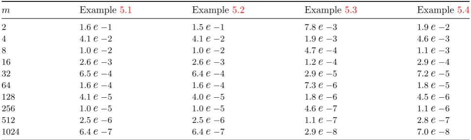
Table 5: Mean-absolute errors, for Examples5.1-5.4, in terms ofm. .

m Example5.1 Example5.2 Example5.3 Example5.4

2 1.6e−1 1.5e−1 7.8e−3 1.9e−2

4 4.1e−2 4.1e−2 1.9e−3 4.6e−3

8 1.0e−2 1.0e−2 4.7e−4 1.1e−3

16 2.6e−3 2.6e−3 1.2e−4 2.9e−4

32 6.5e−4 6.4e−4 2.9e−5 7.2e−5

64 1.6e−4 1.6e−4 7.3e−6 1.8e−5

128 4.1e−5 4.0e−5 1.8e−6 4.5e−6

256 1.0e−5 1.0e−5 4.6e−7 1.1e−6

512 2.5e−6 2.5e−6 1.1e−7 2.8e−7

1024 6.4e−7 6.4e−7 2.9e−8 7.0e−8

Example 5.3 For the following second kind Volterra integral equation [1]:

x(s) + ∫ s

0

(s−t)x(t)t=s, (5.44)

with exact solution x(s) = sin(s), Table 3 shows the numerical results.

Example 5.4 Consider the following second kind Volterra integral equation [14]:

x(s) + ∫ s

0

(st2+s2t)x(t)t=s+ 7 12s

5_{, (5.45)}

with exact solution x(s) = s. Table 4 gives the results.

5.2 Convergence rate

We give here the mean-absolute errors associated with the direct method. The errors are calculated for all the mentioned examples. Table5shows the results for some different values ofm. We see that the direct method has a reasonable convergence rate.

6

Conclusion

A direct method was formulated based on a spe-cial representation of TFs vector forms. This ap-proach, without applying any projection method, transforms a Volterra or Fredholm integral tion of the second kind to a set of algebraic equa-tions. Its efficiency was checked on some exam-ples. The results confirmed the applicability of the method for solving second kind integral equa-tions.

References

[1] E. Babolian, A. Davari, Numerical im-plementation of Adomian decomposition method for linear Volterra integral equations of the second kind,Applied Mathematics and Computation 165 (2005) 223-227.

solving integral equations system using or-thogonal triangular functions, International Journal of Industrial Mathematics 1 (2009) 135-145.

[3] E. Babolian, Z. Masouri, S. Hatamzadeh-Varmazyar, A set of multi-dimensional or-thogonal basis functions and its applica-tion to solve integral equaapplica-tions, Interna-tional Journal of Applied Mathematics and Computation 2 (2010) 032-049.

[4] E. Babolian, Z. Masouri, S. Hatamzadeh-Varmazyar, Introducing a direct method to solve nonlinear Volterra and Fredholm in-tegral equations using orthogonal triangular functions,Mathematics Scientific Journal 5 (2009) 11-26.

[5] E. Babolian, Z. Masouri, S. Hatamzadeh-Varmazyar, New direct method to solve nonlinear Volterra-Fredholm integral and integro-differential equations using opera-tional matrix with block-pulse functions, Progress In Electromagnetics Research B 8 (2008) 59-76.

[6] E. Babolian, Z. Masouri, S. Hatamzadeh-Varmazyar, Numerical solution of nonlinear Volterra-Fredholm integro-differential equa-tions via direct method using triangular functions, Computers & Mathematics with Applications 58 (2009) 239-247.

[7] A. Deb, A. Dasgupta, G. Sarkar, A new set of orthogonal functions and its application to the analysis of dynamic systems,Journal of the Franklin Institute 343 (2006) 1-26.

[8] L. M. Delves, J. L. Mohamed, Computa-tional Methods for Integral Equations, Cam-bridge University Press, CamCam-bridge, 1985.

[9] S. Hatamzadeh-Varmazyar, Z. Masouri, A fast numerical method for analysis of one-and two-dimensional electromagnetic scat-tering using a set of cardinal functions, En-gineering Analysis with Boundary Elements 36 (2012) 1631-1639.

[10] S. Hatamzadeh-Varmazyar, Z. Masouri, De-termining the electromagnetic fields scat-tered from PEC cylinders, International Journal of Mathematics & Computation 28 (2017) 1-8.

[11] S. Hatamzadeh-Varmazyar, Z. Masouri, Numerical expansion-iterative method for analysis of integral equation models aris-ing in one-and two-dimensional electromag-netic scattering, Engineering Analysis with Boundary Elements 36 (2012) 416-422.

[12] S. Hatamzadeh-Varmazyar, M. Naser-Moghadasi, E. Babolian, Z. Masouri, Calculating the radar cross section of the resistive targets using the Haar wavelets, Progress In Electromagnetics Research 83 (2008) 55-80.

[13] S. Hatamzadeh-Varmazyar, M. Naser Moghadasi, R. Sadeghzadeh-Sheikhan, Numerical method for analysis of radiation from thin wire dipole antenna,International Journal of Industrial Mathematics 3 (2011) 135-142.

[14] Z. Masouri, Numerical expansion-iterative method for solving second kind Volterra and Fredholm integral equations using block-pulse functions, Advanced Computational Techniques in Electromagnetics 2012.

[15] Z. Masouri, E. Babolian, S. Hatamzadeh-Varmazyar, An expansion-iterative method for numerically solving Volterra integral equation of the first kind, Computers & Mathematics with Applications 59 (2010) 1491-1499.

[16] Z. Masouri, S. Hatamzadeh-Varmazyar, An analysis of electromagnetic scattering from finite-width strips, International Journal of Industrial Mathematics 5 (2013) 199-204.

[17] Z. Masouri, S. Hatamzadeh-Varmazyar, Evaluation of current distribution induced on perfect electrically conducting scatterers, International Journal of Industrial Mathe-matics 5 (2013) 167-173.

[18] Z. Masouri, S. Hatamzadeh-Varmazyar, Nu-merical solution of Fredholm integral equa-tions of the first kind with real or com-plex kernel using triangular functions, Pro-ceedings of 38th Annual Iranian Mathemat-ics Conference, Zanjan University, Zanjan, Iran (2007) 284-286.

equations, Applied Mathematics and Com-putation 160 (2005) 579-587.

[20] K. Maleknejad, M. Karami, Using the WPG method for solving integral equations of the second kind,Applied Mathematics and Com-putation 166 (2005) 123-130.

[21] K. Maleknejad, M. Tavassoli Kajani, Y. Mahmoudi, Numerical solution of linear Fredholm and Volterra integral equation of the second kind by using Legendre wavelets, Kybernetes 32 (2003) 1530-1539.

Saeed Hatamzadeh-Varmazyar, Ph.D. in Electrical Engineer-ing, is an Assistant Professor at Islamshar Branch, Islamic Azad University, Tehran, Iran. His research interests include computational Electromagnetics, numerical methods for solving integral equations, electromagnetic theory, singular integral equa-tions, electromagnetic radiation and antenna, and propagation of electromagnetic waves, including scattering, diffraction, and etc. Dr. Hatamzadeh-Varmazyar is the author of many research articles published in scientific journals. More details may be found on his official website available online athttp://www.hatamzadeh.ir/

and http://www.hatamzadeh.org/.

Zahra Masouri received her B.Sc., M.Sc., and Ph.D. degrees in Ap-plied Mathematics, respectively, in 1998, 2000, and 2010, as the first rank graduate at all the mentioned educational levels. She is currently an Assistant Professor at Islamshar Branch, Islamic Azad University, Tehran, Iran. Her research interest is in numerical analysis; numerical solution of linear and nonlinear inte-gral, integro-differential, and differential equa-tions; numerical linear algebra; and computa-tional Electromagnetics. Dr. Masouri was the re-search manager and the rere-search vice-chancellor at Khorramabad Branch of Islamic Azad Univer-sity for some years. She also is the author of many research articles published in scientific journals or