Model Predictive Control of a River Reach with Weirs

Model predictive control of a river reach with

weirs

Klaudia Horváth

_{, Bart van Esch}

_{, Jorn Baayen}

_{, Ivo Pothof}

_{, Jan Talsma}

_{and Tjerk Vreeken}

1 _{Eindhoven University of Technology, Eindhoven, The Netherlands} 2 _{KISTERS Nederland B.V., Amersfoort, The Netherlands}

3 _{Deltares, Delft, The Netherlands}

[email protected], [email protected],[email protected], [email protected], [email protected],

[email protected]

Abstract

A decision support system for water management based on convex optimization, RTC-Tools 2, is applied for a water system containing river branches connected by weirs. The advantage of convex optimization is the ability of finding the global optimum, which makes the decision support system robust and deterministic. In this work the convex modeling of open water channels and weirs is presented. The decision support system is implemented for a river made of 12 river reaches divided by movable weirs. It is shown how the discharge wave is dispatched in the river without the water levels exceeding the bounds by controlling the weir heights. After this test the optimization can be applied to a realistic numerical model and model predictive control can be implemented.

1

Introduction

Optimization methods are often used for managing water systems. Model predictive control is one of them and several studies have been carried out about its application [1, 2, 3]. In these studies linear models are used to preserve convexity even though the problem at hand is essentially nonlinear. However, when the nonlinearities are moved to the inequality constraints, it is possible to create a convex optimization problem and in some cases preserve non-linearity of the system. In this research such approach is demonstrated through the modelling of weirs by RTC-Tools 2 [4], a toolbox to create decision support systems, used and applied within the Slim Malen project in cooperation with Deltares and the Dutch Water Boards [5].

* _{Corresponding author}

2

Material and methods

2.1

Modelling

The river branches are modelled with the Integrator Delay model [6]. The water level is the integral of the difference of the in- and outflow. The time it takes for the inflow wave to arrive to downstream is the time delay:

(1) where A is the backwater surface of the river reach, h is the water level and qin and qout are the in-

and outflow rates and τ is the time delay. As Eq. 1 discretized is affine, it can be used as equality constraint (see Eq. 4). The weirs are modelled with the common weir equation:

(2) where Cd is the weir discharge coefficient (approximated as 0.61), g is the acceleration of gravity,

B is the width of the weir, hw is the crest height, and h is the upstream water level. As this equation is

non-linear, it cannot be used as equality constraint.

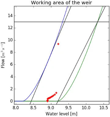
In the optimization problem with controllable weirs, the goal is to find the appropriate crest height so that the constraints (to keep the water level within bounds) are satisfied. The following approach is adopted: in the optimization only the discharge is used and the crest height is calculated as post-processing. However, it should be ensured that all the computed discharges are feasible for the weir: the discharge cannot be larger than the discharge corresponding to the minimum crest level. Thus at each step, the discharge to be calculated is limited by the minimum and maximum discharges that the current water levels and the minimum and maximum crest heights allow. An example for such “working area” of the weir is shown in Figure 1. The possible discharge is bounded by horizontal lines of qmin and qmax: these values should be approximated based on the characteristics of the system.

The left side of the area is bounded by the line corresponding to Eq. 2 with hw =hw,min, when the weir

is in the lowest position (blue line in Figure 1). The area is bounded to the right by the maximum crest height (green line in Figure 1), the line shows the plot of Eq. 2 when hw=hw,max. However, these

relations are non-convex, and therefore their linear approximation is used (black lines in Figure 1). Note that for both lines the approximation is conservative: the approximated area lies completely within the possible non-linear area. This means that any resulting flow-head pair from within the working area has a corresponding crest height that is physically realizable and respects the non-linear weir equation (Eq. 2).

(

)

( )

in out

dh

A q t

q

t

dt

=

- -

t

(

)

2

2

3

d w

-Figure 1: Working area of the weir: with blue and green line the non-linear flow head relations and with black line the actual constraints. The red crosses are the actual head-flow relations during the case study (for weir 1)

Figure 2 Working area of the weir

2.2

Convex optimization approach

The decision support system is using convex optimization which guarantees that the global optimum is reached. This property is crucial for a decision support system. If the problem was not convex, a local optimum can be reached instead, and a small change in the initial conditions might direct the solution into an entirely different local optimum. This fact would reduce the credibility of the decision support system by the user. Therefore, we aim at describing the water system as convex optimization problem in the form [7]:

, (3)

where f0,…,fm are convex functions. The objective and the inequality constraints are convex

functions, but the equality constraints should be affine. The objective can be minimizing energy used by pumps, or minimizing water level error. Constraints can be for example lower and upper bounds within which the water levels should be kept. In case of a water system containing branches and weirs the optimisation problem looks like the following:

( )

( )

minimize

subject to

0

1,...,

1,..., p

T

i i

f x

f x

i

m

a x b

i

£

=

(4) for ever k and for i=1,..,12, where qi-1 is the upstream and qi is the downstream flow of the ith

branch, hi is the water level of the ith branch, A is the backwater area, τk is the integer time delay, hmax

and hmin are the bounds on water level and amax, amin, bmax, bmin are the coefficients of the linear weir

equation corresponding to the minimum and maximum allowable crest level (the equations of the black lines in Figure 1). This example is a feasibility problem: there is no objective function and a solution is valid if the constraints are satisfied, in this case, the water levels are kept within the bounds. Note that each equation contains i and k, thus altogether the optimisation problem of Eq. 4 (in case of considering 16 time steps – or later 16 steps long prediction horizon) has 1152 constraints.

3

Case study

The Linge River is part of the drainage system in the South of the Netherlands. The Upper Linge has 12 branches divided by weirs and the Lower Linge is just one long branch. The Linge is used to collect the water from the polders and lead it to the North Sea through the river Merwede. The water leaves the Linge by free flow or by pumping depending on the water level in the Linge and the Merwede river. The goal of the Slim Malen project is to reduce the cost of pumping. This can be achieved by storing water in the system until the conditions are favourable for free flow.

In this work an optimal strategy for the setting of the weirs is presented in order to use the storage capacity of the Upper Linge. In this work we start with the modelling go the weirs and the pumps are modelled in later stage of the project. This is carried out by mathematical optimisation, by using the RTC-Tools 2. The Upper Linge contains 12 branches separated by weirs. There is an inflow upstream and this example a fixed outflow (0.1m3_{/s) downstream. The characteristics of the weirs together with}

the geometry of the system, including the calculated time delay, are shown in Table 1. The backwater area and the time delay is obtained from [8]. The time step for the control is 30 minutes.

Branch name

Backwater area

(m2_{) (Time step)} Delay Min. crest level _(m) Max. crest level _{(m) width} Weir

(m)

( )

( )

( )

( )

( )

( )

find

subject to

( )

( )

(

1) h (k)

(k)

(k

)

i i i

i i i

i i

i i

i i

i i

i i i i ki

i i

x

q k

a

h k

b

a

h k

b

q k

q

q k

q k

q

h

h k

h k

h

t

t

h k

q

q

A

A

t

-Branch 7 270461 1 5.51 6.01 5.94

Branch 8 55691 0 4.8 5.72 5.94

Branch 9 99111 1 3.72 4.58 6.0

Branch

10 436163 3 2.42 3.35 9.5

Branch

11 103840 1 1.47 2.26 9.5

Branch

12 210146 1 - - -

Table 1: Geometry of the branches and the weirs, data is obtained from [8]

4

Results and discussion

4.1

Results

The following test illustrates how the optimisation procedure works. The system has an upstream inflow with a step at 2 hours (Figure 2) and a constant outflow downstream (0.5m3/s). The goal of the decision support system is to propose weir movements such that the water level stays within the prescribed bounds in all reaches. There was one optimisation step carried out (no receding horizon was used), thus the coming disturbance is known by the controller. The resulting water and weir levels and the corresponding discharges are shown for each branch in Figure 3-8.

Figure 3 shows the results in the first two branches. It can be seen that the weir crest is lowered as soon as the inflow wave arrived so that the water level could stay within the bounds. Similar action is seen for branch 3 and 4 (Figure 4). The height of the wave decreases as it moves to the next branch. Branch 6 is the first one with delay, it can be seen that the weir crest height starts to decrease half an hour after the upstream perturbation (Figure 5). The attenuated wave is sent through the branches. The water levels in the downstream branches hardly change; the presence of the wave can be seen by the weir movements and the outflow (Figure 6). Branch 9 has 1.5 hours of delay (Figure 7), thus the discharge wave arrives there at 5th hour of the simulation (3 hours after the upstream perturbation). Half an hour later the wave arrives to the last two branches (Figure 8). The water levels again stay close to constant, at the lower end of the allowable water level bounds. By the end of the simulation the water volume is distributed along the branches, Branch 4 has slightly more water level increase than the other branches.

Figure 5: Water levels (grey) with weir height (black) and discharge in branches 5 and 6

5

Conclusions

A decision support system, RTC-Tools 2, based on convex optimization is presented. The convex modelling of open water channels and weirs is described. The system is illustrated through a case study with a river containing 12 reaches divided by weirs. It was shown that by applying the weir movements calculated by the decision support system, the water levels can be kept within the prescribed bounds. After this test the optimization can be applied to a realistic numerical model and model predictive control can be implemented.

ACKNOWLEDGEMENT

This research is carried out within the Slim Malen project. The Slim Malen (Smart Drainage) project is funded and performed by the following partners: STOWA, Ministry of Economic Affairs (RVO), Deltares, Eindhoven University of Technology, Ministry of Infra and Environment (Rijkswaterstaat – WVL), Water Authorities Hoogheemraadschap Hollands Noorderkwartier, Fryslân, Zuiderzeeland, Rivierenland, Scheldestromen, Rijnland, Brabantse Delta and Hollandse Delta and by companies Nelen & Schuurmans, e-Risk Group, Eneco, Delta, Alliander EXE, Actility, XYLEM and Kisters.

References

[1] Rodellar, J., Gómez, M., and Martín Vide, J. P., Stable predictive control of open-channel flow. Journal of Irrigation and Drainage Engineering, (1989) 115(4):701-713.

[2] Wahlin, B. T., Performance of model predictive control on ASCE Test Canal 1, Journal of Irrigation and Drainage Engineering, (2004)130(3):227-238.

[3] van Overloop, P.-J., Model predictive control on open water systems. PhD thesis, Delft University of Technology, Delft, The Netherlands, 2006.

[4] Gijsbers, P.J.A., Baayen, J.H., ter Maat, G.J.: Quick scan tool for water allocation in the Netherlands. In: Environmental Software Systems, ISESS 2017 (2017)

[5] Slim Malen Project: www.slimmalen.nl

[6] Schuurmans, J., Bosgra, O. H., & Brouwer, R., Open-channel flow model approximation for controller design. Applied Mathematical Modelling, (1995) 19(9), 525-530.

[7] Boyd, Stephen, and Lieven Vandenberghe, Convex optimization, Cambridge university press, 2004.