Mean value theorem for integrals and its application on numerically solving of Fredholm integral equation of second kind with Toeplitz plus Hankel ‎Kernel

(1)

Vol. 6, No. 4, 2014 Article ID IJIM-00402, 10 pages Research Article

Mean value theorem for integrals and its application on numerically

solving of fredholm integral equation of second kind with Toeplitz

plus Hankel Kernel

N. Mikaeilvand ∗†, S. Noeiaghdam ‡

————————————————————————————————–

Abstract

The subject of this paper is the solution of the Fredholm integral equation with Toeplitz, Hankel and the Toeplitz plus Hankel kernel. The mean value theorem for integrals is applied and then extended for solving high dimensional problems and finally, some example and graph of error function are presented to show the ability and simplicity of the method.

Keywords : Fredholm Integral Equations; Toeplitz plus Hankel Kernel; Mean Value Theorem for Integrals.

—————————————————————————————————–

1 Introduction

T

hkel or Toeplitz plus Hankel kernel attractse integral equations with a Toeplitz, Han-attention of many authors as they have practi-cal applications in such diverse fields as scatter-ing theory, fluid dynamics, linear filterscatter-ing the-ory, and inverse scattering problems in quantum-mechanics, problems in radiative wave transmis-sion, and further applications in Medicine and Bi-ology [1,2,6,7, 8,11,15,18,19,20, 21].

Many different powerful methods have been proposed to obtain exact and approximate so-lution of integral equation with a Toeplitz plus Hankel kernel. Solvability of the integral equa-tions with TPH kernel considered in ([12] ). Fred-holm integral equations with TPH kernel have been solved numerically in ([13]). Also, Fredholm

∗_{Corresponding author. [email protected]} †_{Department of Mathematics, Ardabil Branch, Islamic}

Azad University, Ardabil, Iran.

‡_{Young Researchers and Elite Club, Tabriz Branch,}

Is-lamic Azad University, Tabriz, Iran.

integral equations solved by variational iteration method ([17]), homotopy perturbation method (HPM) ([5,14]), Adomian decomposition method (ADM) ([4,9]).

In [3], Avazzadeh et al. introduced a new method for solving Fredholm integral equation by using integral mean value method (IMVM)and M. Heydari et al. [10] extended their method for high dimensional Fredholm integral equations. Based on their works, in this paper, (IMVM) is used for solving integral equations with Toeplitz, Hankel and Toeplitz plus Hankel kernel.

The paper organized as follow : Section2 intro-duces the main idea of method for solving Fred-holm integral equation with TPH kernel and also, some exampels, graph of error function and com-parison between exact and approximate solution for one dimensional Fredholm integral equations with TPH kernel. Our idea is devoted to general-ized the method for solving two and also, high di-mensional integral equations in Sections3 and4. Section4, includes the extented formulae to clar-ify the generalization process and some numerical

(2)

example, graph of error functions and compari-son between exact and approximate solution to describe the method, and Section 5 is discussion and conclusion.

2 Fredholm integral equation

with TPH kernel

Consider the following nonlinear Fredholm inte-gral equation of second kind:

u(x) =f(x)+λ ∫ b

a

[P(x−t)+Q(x+t)]F(u(t))dt, (2.1) whereλ is a real number and also F, f, P and Q are given continuous functions, anduis unknown function to be determined.

For solving TPH kernel with IMVM, we use mean value theorem for integrals as follows:

Theorem 2.1 (mean value theorem for integrals [22]). If w(x) is continuous in [a, b], then there is a point c∈[a, b], such that

∫ b

a

w(x)dx= (b−a)w(c), (2.2)

Now, we illustrate the main idea of our method. By applying the above theorem to Eq. (2.1) we have

u(x) = f(x) +λ(b−a)

[p(x−c) +q(x+c)]F(u(c)), c ∈ [a, b]

(2.3)

now we must just find c and u(c) as unknowns. Substitution ofc into Eq. (2.3)

u(c) =f(c) +λ(b−a)[p(0) +q(2c)]F(u(c)) (2.4)

For constructing another equation concerning c and u(c) we substitute Eq. (2.3) into Eq. (2.1)

u(x) = f(x) +λ ∫ b

a

[p(x−t) +q(x+t)]

F(f(t) +λ(b−a)[p(t−c)

+q(t+c)]F(u(c)))dt (2.5)

substitutingx=c in to (2.5):

u(c) = f(c) +λ ∫ b

a

[p(c−t) +q(c+t)]

F(f(t) +λ(b−a)[p(t−c)

+q(t+c)]F(u(c)))dt (2.6)

Now, we solve Eqs. (2.4) and (2.6) simultane-ously. For solving the above nonlinear system, various methods can be used.

Some different examples of Fredholm integral equation with Toeplitz, Hankel and Toeplitz plus Hankel kernel are chosen to illustrate the pre-sented method. The results show the ability and simplicity of the method.

Example 2.1 ( Fredholm integral equation with Toeplitz kernel): Consider the integral equations

u(x) = 1

3(−1 +e)e

x₊_e2x₋ 1

3 ∫ 1

0

ex−tu(t)dt

for which the exact solution is u(x) =e2x. Using the presented method leads to the following system of equations:

  

u(c) = 1₃(−1 +e)ec+e2c−1₃u

u(c) = (−₃1 +e₃)ec+e2c+ 1₃((4₃ +4₃e)ec+1₃u) By mentioned method, values of c and u(c) are found as follows:

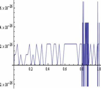
c= 0.5413248546, u(c) = 2.9524924420 Hence, we have u(x) = e2x −1.11022×10−16. The error function is demonstrated in Figure 1.

Note that the absolute error is−1.11022×10−16 with considering 16 digits and it is equivalent to the exact solution.The comparison between ex-act solution and approximate solution showned in Figure 2.

Example 2.2 (Fredholm integral equation with Hankel kernel):

u(x) =−(−2 +e)ex+x2+ ∫ 1

0

ex+tu(t)dt

for which the exact solution is u(x) = x2_.Using the presented method leads to the following system of equations:

      

u(c) =c2+ (2−e)ec+e2cu

u(c) =c2+ (2 +e)ec+1₂ec

(3)

Figure 1: The error function of Example

2.1.

Figure 2: The comparison between exact solution and approximate solution of Exam-ple2.1.

Solving the obtained system leads to

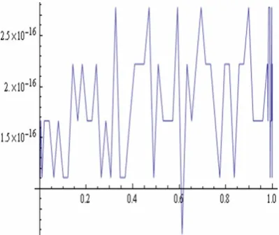
c= 0.5413248546, u(c) = 2.9524924420 with considering 10-digit accuracy.Hence, approx-imate solution isu(x) =x2−4.12812×10−16 and absolute error is −4.12812×10−16. In Figure 3. show the comparison between exact solution and approximate solution and The error function is demonstrated in Figure 4.

Example 2.3 ( Fredholm integral equation with TPH kernel):

u(x) = x3−2(3 + cos(1)−4 sin(1)) × (cos(x) + sin(x))

+ ∫ 1

0

[sin(x+t) + cos(x−t)]u(t)dt

for which the exact solution isu(x) =x3.and

sys-Figure 3: The error function of Example

2.2.

tem of equations is: 

                         

u(c) =c3−2(3 + cos(1)−4 sin(1)) (cos(c) + sin(c))

−1/2(cos(c) + sin(c))

(4(3 + cos(1)−4 sin(1)) sin(1)2 +u(−3 + cos(2))(cos(c) + sin(c)))

u(c) =c3−2(3 + cos(1)−4 sin(1)) (cos(c) + sin(c))

+(sin(c+c) + cos(c−c))u(c)

By solving of the related system, we have

c= 0.6296960723676109

and

u(c) = 0.6296960723676109.

(4)

10−16_{. Figure}₅ _{is comparison between exact and} approximate solution and The error function is demonstrated in Figure 6.

2.3.

3 Solving of two dimensional

Fredholm

integral

equation

with TPH kernel via IMVM

Consider the following two dimensional Fredholm integral equation of the second kind:

u(x, y) = f(x, y) +λ ∫ b

a

∫ d

c

(P[(x, y)−(s, t)]

+Q[(x, y) + (s, t)]F(u(s, t))dsdt

(3.7)

For solving the above equation, we apply the in-tegral mean value theorem. However, the mean value theorem is valid for double integrals, we apply one dimensional integral mean value theo-rem directly to fulfill required linearly indepen-dent equations.

Corollary 3.1 (mean value theorem for inte-grals). If w(x, y) is continuous in [a, b]×[c, d], then there are points c1 ∈ [a, b] and c2 ∈ [c, d], such that

∫ b

a

w(s, t)ds= (b−a)w(c1, t) (3.8)

and _∫

d

c

w(s, t)dt= (d−c)w(s, c2) (3.9)

Proof:It is clear by using(2.2)

Theorem 3.1 (mean value theorem for double integrals). Ifw(x, y)is continuous in[a, b]×[c, d], then there are points c1 ∈ [a, b] and c2 ∈ [c, d], such that

∫ b

a

∫ d

c

w(s, t)dsdt= (b−a)(d−c)w(c1, c2). (3.10) Proof: It is clear using Theorem (2.1).

By applying (3.8) and (3.9) for the right hand of (3.7), since the integral equation (3.7) depends on x and y, c1 and c2 will be functions with respect to x and y and here we write them as c1(x;y))∈[a, b] andc2(x;y))∈[c, d]. To be able to implement our algorithm, we takec1(x;y)) and c2(x;y)) as constants. Now to find the solution of integral equation we describe the following al-gorithm:

Algorithm

1. Apply (3.9) in (3.7) to get

u(x, y) =f(x, y) +λ(d−c)∫_ab(P[(x, y) −(s, c2)] +Q[(x, y) + (s, c2)])F(u(s, c2)))ds

(3.11)

2. Apply (3.8)in (3.11)and Replace the ob-tained equation in 3.11as

u(x, y) =f(x, y) +λ(b−a)(d−c) (P[(x, y)−(c1, c2)] +Q[(x, y) + (c1, c2)])

F(u(c1, c2))

(5)

3. Let (x, y) = (c1, c2)in the (3.12). It is ob-tained as

u(c1, c2) =f(c1, c2) +λ(b−a)(d−c) (P[(c1, c2)−(c1, c2)] +Q[(c1, c2)

+(c1, c2)])F(u(c1, c2))

(3.13)

4. Replace (3.12) into (3.7) and then let(x, y) = (c1, c2) in the obtained formula.

u(c1, c2) =f(c1, c2) +λ∫_ab∫_cd(P[(c1, c2) −(s, t)] +Q[(c1, c2) + (s, t)])F(f(s, t)

+λ(b−a)(d−c)(P[(s, t)−(c1, c2)] +Q[(s, t) + (c1, c2)])F(u(c1, c2)))dsdt

(3.14)

5. Substitute (3.12) into (3.11). We have

u(x, y) =f(x, y) +λ(d−c)∫_ab(P[(x, y) −(s, c2)] +Q[(x, y) + (s, c2)]F(f(s, c2) +λ(b−a)(d−c)(P[(s, c2)−(c1, c2)] +Q[(s, c2) + (c1, c2)])F(u(c1, c2)))) ds

(3.15)

6. Let(x, y) = (c1, c2) to be in the above equa-tion

u(c1, c2) =f(c1, c2) +λ(d−c) ∫b

a(P[(c1, c2)

−(s, c2)] +Q[(c1, c2) + (s, c2)])F(f(s, c2) +λ(b−a)(d−c)(P[(s, c2)−(c1, c2)] +Q[(s, c2) + (c1, c2)])F(u(c1, c2)))ds

(3.16)

7. Solve the Eqs. (3.13), (3.14) and (3.16) si-multaneously as the system including 3 equa-tions and 3 unknownsc1;c2 and u(c1, c2).

4 Solving of high dimensional

integral equations via IMVM

Consider the second kind high dimensional inte-gral equation

u(x) =f(x) +λ∫b1

a1 ∫b2

a2 ... ∫bn

an[P(x−t)

+Q(x+t)]F(u(t))dt

(4.17) where x = (x1, x2, ..., xn) and t = (t1, t2, ..., tn).

Similar to the previous section, instead of using mean value theorem for multiple integral, we ap-ply one dimensional integral mean value theorem directly to provide needful linearly independent equations.

Theorem 4.1 (mean value theorem for multiple integrals): If s(x) is continuous in [ai, bi]n, i =

1,2, ..., n, then there are points ci ∈ [ai, bi], i =

1,2, ..., n such that ∫b1

a1 ∫b2

a2 ... ∫bn

an(s(x)) dxn dxn−1 ... dx1

=∏n_j₌₀−1(bn−j−an−j)s(c1, c2, ..., cn)

(4.18) In the similar way, to find u(x1, x2, ..., xn), we

have to obtain c1, c2, ..., cn and u(c1, c2, ..., cn).

Follow the consecutive substituting in the follow-ing algorithm which lead to the system includfollow-ing (n+1) unknowns and (n+1) linearly independent equations.

Algorithm

1. Apply the integral mean value theorem for interval[an, bn]:

∫bn

an[p(x−t) +q(x+t)]F(u(t))dtn

= (bn−an)[p(x−ξn) +q(x+ξn)]F(u(ξn))

(4.19) whereξn= (t1, t2, ..., tn−1, cn).

2. Substitute (4.19) into (4.17) to obtain :

u(x) =

f(x) +λ(bn−an)

∫b1

a1 ... ∫bn−1

an−1[p(x−ξn) +q(x+ξn)]F(u(ξn))dtn−1· · ·dt1

(4.20)

3. Again, we use the integral mean value theo-rem withi=n−1,as follows

∫bn−1

an−1[p(x−ξn) +q(x+ξn)]F(u(ξn))dtn−1 = (bn−1−an−1)[p(x−ξn−1) +q(x

+ξn−1)]F(u(ξn−1))

(4.21) whereξn−1 = (t1, t2, ..., cn−1, cn).

4. Replace the above equation into (4.20). So, we have

u(x) =_∫f(x) +λ(bn−an)(bn−1−an−1) b1

a1 · · · ∫bn−2

an−2[p(x−ξn−1) +q(x+ξn−1)]F(u(ξn−1))dtn−2· · ·dt1

(4.22)

5. Repeat the process fori= 3, ..., n−1, as

u(x) =f(x) +λ(bn−an)· · ·(bn−i+1 −an−i+1)

∫b1

a1 · · · ∫bn−i

an−i[p(x−ξn−i+1)

(6)

where ξn−i+1 = (t1, t2, ..., tn−i, cn−i+1, cn−i+2, ..., cn). Also,

the nth step of the above process leads to

u(x) = f(x) +λ(bn−an)· · ·(b1−a1)

[p(x−ξ1) +q(x+ξ1)]F(u(ξ1)) (4.24)

where ξ1= (c1, c2, ..., cn).

6. Letx=ξ1 into4.24to get

u(ξ1) = f(ξ1) +λ

n

∏

j=1

(bj−aj)[p(0)

+q(2ξ1)]F(uξ1)) (4.25)

Now the first equation of the proposed sys-tem including (n+ 1)unknowns and (n+ 1) equations is constructed.

7. To make the other equations, the demon-strated process must be repeated such that the ith achieved equation is as follows (use (4.23) and (4.24))

u(x) =

f(x) +λ∏i_j−₌₀1(bn−j−an−j)

∫b1

a1 · · · ∫bn−i

an−i

[p(x−ξn−i+1) +q(x+ξn−i+1)]

F([f(ξn−i+1) +λ

∏i−1

j=0(bn−j−an−j)

[p(0) +q(2ξn−i+1)]F(u(ξ1))])dtn−i· · ·dt1 (4.26)

wherei= 1, ..., n−1 , and gives u(ξ1) =

f(ξ1) +λ∏i_j−₌₀1(bn−j−an−j)

∫b1

a1 ... ∫bn−i

an−i

[p(ξ1−ξn−i+1) +q(ξ1+ξn−i+1)]

F([f(ξn−i+1) +λ

∏i−1

j=0(bn−j −an−j) [p(ξn−i+1−ξ1) +q(ξn−i+1+ξ1)]

F(u(ξ1))])dtn−i· · ·dt1

(4.27)

as the ith equation. Therefore, we obtain the (n−1), new equations when i = 1, ..., n− 1,for final mentioned system including (n+ 1)unknowns and (n+1) equations. Also,4.25 can be provided4.27 withi=n.

8. Implement the previous step to obtain the nth equation as

u(x) = f(x) +λ ∫ b1

a1 · · ·

∫ bn

an

[P(x−t) +q(x+t)]

F(f(t) +λ

n∏−1

j=0

(bn−j −an−j)

[p(t−ξ1) +q(t+ξ1)] F(u(ξ1)))dtn· · ·dt1

(4.28)

which lead to

u(ξ1) = f(ξ1) +λ ∫ b1

a1 · · ·

∫ bn

an

[P(ξ1−t) +q(ξ1+t)]

F(f(t) +λ

n_∏−1

j=0

(bn−j−an−j)

[p(t−ξ1) +q(t+ξ1)] F(u(ξ1)))dtn· · · dt1

(4.29)

Finally, the last equation of the proposed system including (n+ 1) unknowns and (n+ 1) equations is constructed.

9. Solve the nonlinear system including (4.25), (4.27) and (4.29) with the Newtons method or other efficient methods.

Remark 4.1 The equations of the final system include the numerous integrals containing long terms. It is recommended to use the numerical integration rules such as Gauss quadrature rule or trapezoidal integration method.

Some different examples of two dimensional Fredholm integral equation with Toeplitz ,Han-kel and Toeplitz plus Han,Han-kel kernel are chosen to illustrate the presented method.

Example 4.1 ( Two dimensional Fredholm in-tegral equation with Hankel kernel) Consider the integral equations:

u(x, y) =f(x, y) + ∫ 1

0 ∫ 1

0

2x+y+s+tu(s, t) ds dt

where

f(x, y) =x+y−2

x+y₍₋_{2 + log(16))}

(7)

for which the exact solution is u(x, y) = x+y. Using the presented method leads to the following system of equations:

u(c1, c2) =

c1+c2+ 1 log(2)4 2−

1+c1+c2

(2c2log(2)3+ 3×2c1+2c2ulog(2)3 +2(−3×2c2 _{+ log(2)}2₎₍−_{1 + log(4)))}

−2c1+c2(−2 + log(16)) log(2)3

u(c1, c2) =

c1+c2−

2c1+c2₍−_{2 + log(16))} log(2)3

+ 1 log(2)52−

2+c1+c2₍₉×₂c1+c2_u(c

1, c2) log(2)3 +(−2 + log(16))(−9 + log(2) log(16)))

u(c1, c2) = c1+c2− 2

c₁₊c₂₍₋_2+log(16))

log(2)3 +2c1+c2+c1+c2_u(c

1, c2)

By mentioned method, values of c1, c2and u(c1, c2) are found as

c1 = 0.5449840956, c2 = 0.5449055202

and

u(c1, c2) = 2.9524924420

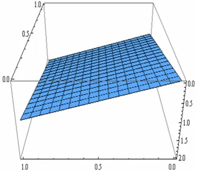
. Hence, u(x, y) =x+y+ 3.55271×10−15 . The error function is demonstrated in Figure 7. Note that the absolute error is 3.55271×10−15 with considering 15 digits and it is equivalent to the exact solution.The comparison between exact solution and approximate solution showned in Figure 8.

Example 4.2 ( Two dimensional Fredholm integral equation with Toeplitz kernel)

u(x, y) =f(x, y)+ ∫ 1

0 ∫ 1

0

e(2x+2y)−(s+t)u(s, t)ds dt

where

f(x, y) =x−y

Figure 7: The error function of Example .

Figure 8: The comparison between exact solution and approximate solution of Exam-ple .

for which the exact solution is u(x, y) = x−y. Using the presented method leads to the following system of equations:

u(c1, c2) = c1−c2+e−1+c1+c2_(ec1

(−2 +c2+e−c2e) + (−1 +e) e1+c2_u(c

1, c2)),

u(c1, c2) = c1−c2+ (−1 +e)2ec1+c2 u(c1, c2),

u(c1, c2) = c1−c2+e(2c1+2c2)−(c1+c2) u(c1, c2).

Solving the obtained system leads to

(8)

and

u(c1, c2) =−2.9338723141×10−27

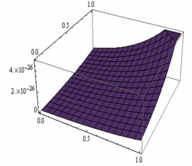
with considering 10-digit accuracy.Hence, approx-imate solution isu(x, y) =x−y+6.94271×10−26 and absolute error is6.94271×10−26.In Figure9. show he comparison between exact solution and approximate solution and The error function is demonstrated in Figure 10.

4.2.

Example 4.3 ( Two dimensional Fredholm in-tegral equation with TPH kernel)

u(x, y) = f(x, y) + ∫ 1

0 ∫ 1

0

(e(2x+2y)−(s+t)

+e(x+y)+(s+t) u(s, t) ds dt

where

f(x, y) =x2−y2

for which the exact solution is u(x, y) = x2 − y2.and system of equations is:

u(c1, c2) = c2₁−c2₂+1 6e

−1+c2

(−6(5 +c2₂(−1 +e)−2e)e2c1 +3e1+2c1+3c2₍−_{1 +}_e2_)u(c

1, c2) + 2e1+2c2 (−1 +e3+ 3e3c1)u(c1, c2)

−6e1+c1+c2_{(2 +}_c2

2(−1 +e) +u(c1, c2)−e(1 +u(c1, c2)))),

u(c1, c2) = c21−c22+ 1

36(36(−1 +e) 2

ec1+c2 _{+ 36e}3(c1+c2)_{+ 9e}2 (c1+c2)(−1 +e2)2+ 4 (−1 +e3)2)u(c1, c2),

u(c1, c2) = c21−c22+ (e(2c1+2c2)−(c1+c2) +ec1+c2+c1+c2_)u(c

1, c2).

By solving of the related system, we have

c1= 0.6114976933, c2 = 0.6114976933

and

u(c1, c2) = 5.6991080150×10−21

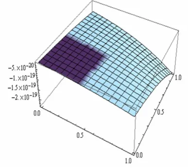
Hence, approximate solution isu(x, y) = (x2− y2₎ ₋ _2.34655 _× ₁₀−19 _{and absolute error is} −2.34655×10−19. Figure 11. is comparison be-tween exact and approximate solutions and The error function is demonstrated in Figure 12.

Acknowledgements

This work has been supported by Islamic Azad University, Ardabil branch, research grand.

5 Conclusions

(9)

4.3.

Toeplitz plus Hankel kernel.We exhibit the ap-plied main idea that it just is the famous integral mean value theorem. Exampels that were pre-sented show the ability of the model. The results confirm that the method is very effective and sim-ple.

References

[1] Z. S. Agranovich, V. A. Marchenko,The In-verse Problem of Scattering Theory, Gordon Breach, New York, 1963.

[2] G. B. Arfken, H. J. Weber, F. E. Har-ris, Mathematical Methods for Physicists, A Comprehensive Guide, seventh ed., Aca-demic Press, Amsterdam”NewYork”Tokyo, 2012.

[3] Z. Avazzadeh, M. Heydari, G. B. Logh-mani, Numerical solution of Fredholm inte-gral equations of the second kind by using integral mean value theorem, Appl. Math. Model. 35 (2011) 2374- 2383.

[4] E. Babolian, J. Biazar, A. R. Vahidi, The decomposition method applied to systems of Fredholm integral equations of the second kind, Appl. Math. Comput. 148 (2004) 443-452.

[5] J. Biazar, H. Ghazvini, Numerical solution for special nonlinear Fredholm integral equa-tion by HPM, Appl. Math. Comput. 195 (2008) 681-687.

[6] A. Bttcher, B. Silbermann, Analysis of Toeplitz Operators, Springer Monographs in Mathematics, Springer-Verlag, Berlin, 2006.

[7] K. Chanda, P. C. Sabatier,Inverse Problems in Quantum Scattering Theory, Springer-Verlag, New York, 1989.

[8] F. Garcia-Vicente, J. M. Delgado, C. Ro-driguez,Exact analytical solution of the con-volution integral equation for a general pro-file fitting function and Gaussian detector kernel, Phys. Med. Biol. 45 (2000) 645-650.

[9] A. Gorguis,Charpit and Adomian for solving integral equations, Appl. Math. Comput. 193 (2007) 446 - 454.

[10] M. Heydari, Z. Avazzadeh, H. Navabpour, G. B. Loghmani,Numerical solution of Fred-holm integral equations of the second kind by using integral mean value theorem II. High dimensional problems, Appl. Math. Model. Vol. 37 (2013) 432-442.

[11] T. Kailath, L. Ljung, M. Morf, Generalized KreinLevinson equations for efficient calcu-lation of Fredholm resolvents of nondisplace-ment kernels, Topics in Functional Analysis, Adv. Math. Suppl. Stud., vol. 3, Academic Press, New York” London, 1978.

(10)

[13] K. Maleknejad, M. Rabbani, Numerical so-lution for the Fredholm integral equation of the second kind with Toeplitz kernels by using preconditioners, Appl. Math. Comput. 180 (2006) 128-133.

[14] J. S. Nadjafi, A. Ghorbani, Hes homo-topy perturbation method: an effective tool for solving nonlinear integral and integro-differential equations, Comput. Math. Appl. 58 (2009) 2379-2390.

[15] K. J. Olejniczak, The Hartley transform, A. D. Poularikas (Ed.), The Transforms and Applications Handbook, third ed., The Elec-trical Engineering Handbook Series, Part 4, CRC Press with Taylor and Francis Group, Boca Raton London New York, 2010.

[16] A. Razani, Z. Goodarzi, A Solution of Volterra-Hamerstain Integral Equation in Partially Ordered Sets, Int. J. Industrial Mathematics 3 (2011) 277-281.

[17] R. Saadati, M. Dehghan, S. M. Vaezpour, M. Saravi, The convergence of Hes varia-tional iteration method for solving integral equations, Comput. Math. Appl. 58 (2009) 2167-2171.

[18] I. SenGupta, Differential operator related to the generalized superradiance integral equa-tion, J. Math. Anal. Appl. 369 (2010) 10-21.

[19] I. SenGupta, B. Sun, W. Jiang, G. Chen, M. C. Mariani, Concentration problems for bandpass lters in communication theory over disjoint frequency intervals and numerical solutions, J. Fourier Anal. Appl. 18 (2012) 182-210.

[20] E. C. Titchmarsh, Introduction to the The-ory of Fourier Integrals, Chelsea, New York, 1986.

[21] J. N. Tsitsiklis, B. C. Levy, Integral Equa-tions and Resolvents of Toeplitz Plus Han-kel Kernels, Technical Report LIDS-P-1170, Laboratory for Information and Decision Systems, M.I.T., silver ed., December 1981.

[22] R. A. Silverman,Essential Calculus with Ap-plications, Dover, 1989.

Nasser Mikaeilvand is Assistance Professor of applied mathematics at Ardabil branch, Islamic Azad University, Ardabil, Iran. In-terested in numerical solutions of Differential and Integral Equa-tions, numerical linear algebra and Fuzzy mathematics.