Comparison of confidence interval methods for an intra-class correlation coefficient (ICC)

R E S E A R C H A R T I C L E

Open Access

Comparison of confidence interval methods for an

intra-class correlation coefficient (ICC)

Alexei C Ionan

, Mei-Yin C Polley

, Lisa M McShane

and Kevin K Dobbin

Abstract

Background:The intraclass correlation coefficient (ICC) is widely used in biomedical research to assess the

reproducibility of measurements between raters, labs, technicians, or devices. For example, in an inter-rater reliability study, a high ICC value means that noise variability (between-raters and within-raters) is small relative to variability from patient to patient. A confidence interval or Bayesian credible interval for the ICC is a commonly reported summary. Such intervals can be constructed employing either frequentist or Bayesian methodologies.

Methods:This study examines the performance of three different methods for constructing an interval in a two-way, crossed, random effects model without interaction: the Generalized Confidence Interval method (GCI), the Modified Large Sample method (MLS), and a Bayesian method based on a noninformative prior distribution (NIB). Guidance is provided on interval construction method selection based on study design, sample size, and normality of the data. We compare the coverage probabilities and widths of the different interval methods.

Results:We show that, for the two-way, crossed, random effects model without interaction, care is needed in interval method selection because the interval estimates do not always have properties that the user expects. While different methods generally perform well when there are a large number of levels of each factor, large differences between the methods emerge when the number of one or more factors is limited. In addition, all methods are shown to lack robustness to certain hard-to-detect violations of normality when the sample size is limited. Conclusions:Decision rules and software programs for interval construction are provided for practical

implementation in the two-way, crossed, random effects model without interaction. All interval methods perform similarly when the data are normal and there are sufficient numbers of levels of each factor. The MLS and GCI methods outperform the NIB when one of the factors has a limited number of levels and the data are normally distributed or nearly normally distributed. None of the methods work well if the number of levels of a factor are limited and data are markedly non-normal. The software programs are implemented in the popular R language.

Keywords:Confidence interval, Credible interval, Generalized confidence interval, Intraclass correlation coefficient, Modified large sample

Background

Biological and physical quantities assessed for scientific studies must be measured with sufficient reproducibility for the study to produce meaningful results. For example, biological markers (“biomarkers”) are studied for many medical applications, including disease risk prediction, diagnosis, prognosis, monitoring, or optimal therapy selec-tion. Variation in measurements occurs for numerous rea-sons. The measurements might have been made on

different devices, may have involved subjective judgment of human raters (e.g., a pathologist assessing the number of tumor cells in a biopsy), or might have been made in different laboratories using different procedures. As an-other example, psychological instruments often score pa-tients based on multi-item questionnaires completed by medical professionals. Variation in the resulting scores can be attributed to both variation among the patients and variation among the medical professionals performing the assessments. In many settings, it is not realistic to expect perfect concordance among replicate measurements, but one needs to achieve a level of reliability sufficient for the

* Correspondence:[email protected] 3

Department of Epidemiology and Biostatistics, University of Georgia, Athens, GA, USA

Full list of author information is available at the end of the article

application area, such as a clinical setting. A common approach to quantify the reliability of a measurement process is to calculate the intraclass correlation coefficient (ICC) along with a confidence interval [1-4].

An interval can be constructed for the ICC using fre-quentist or Bayesian methods. Frefre-quentist methods as-sure that the probability that the interval contains the parameter if the experiment is repeated many times is the nominal confidence level (e.g., 95%). In contrast to Frequentist methods, Bayesian methods provide a prob-ability distribution for the parameter itself, given the data and the prior uncertainty. The distribution can be summarized by a credible interval, which reflects a nom-inal probability (e.g., 95%) region for the distribution. When little is known about the parameter of interest a priori, then a non-informative prior, which is often pro-vided in the statistical software, can be used to construct the interval. The relative advantages of noninformative Bayesian and frequentist approaches in general are dis-cussed in Berger [5] Chapter 4, Carlin and Louis [6] (Section 1.4), and elsewhere. General comparisons of the different approaches are beyond the scope of this paper. This paper focuses on two issues of applied interest dis-cussed in the next paragraph.

Two critical and inter-related characteristics of a confi-dence interval method are (1) the coverage probability, and (2) the interval width. The coverage probability of a method should exactly match the confidence level, such as 95%. Coverage probability is a frequentist concept since the parameter is treated as a fixed number. The interval width is important to consider when comparing intervals because one often wants the shortest possible interval that maintains the nominal coverage. Coverage probability and interval width are important and relevant from both frequentist and objective Bayesian perspectives [7-13]. Fre-quentist coverage probabilities are interpretable in the Bayesian framework as well [14].

We study two applications in detail. The first applica-tion is a study by Barzman et al. [15]. They evaluated the Brief Rating of Aggression by Children and Adolescents (BRACHA), a 14-item questionnaire instrument scored by emergency room staffers. BRACHA scores can be influ-enced by both the child being assessed and the adult per-forming the assessment. Interest was in whether different adult staffers scored the children in a similar way, as sum-marized by the intraclass correlation coefficient. These data were originally analyzed using Bayesian credible interval methods. The second application is the National Cancer In-stitute’s Director’s Challenge reproducibility study [16]. In this study, tissue samples were subdivided into separate sec-tions, sections distributed to four laboratories, and micro-array analysis performed at each laboratory. Interest was in whether different laboratories produced similar gene ex-pression measurements for individual patients.

This paper considers the setting of a two factor, crossed, random effects model without interaction. We focus on this setting because it arises frequently in practical applica-tions of interest [15-17], and because this focus enables us to examine different aspects of study design, data distribu-tion, and Bayesian priors, without the scope of the paper becoming unwieldy. For the purposes of this study, we as-sume this model is appropriate for the data; the process of selecting an appropriate statistical model and agreement measure are outside the scope of this paper and are dis-cussed thoroughly elsewhere [18,19]. A random effects model is appropriate when each factor represents a ran-dom sample from a larger population [20]; for example, a factor may represent labs randomly drawn from all labs that could perform the assay. If the population of labs is small, a finite population adjustment is possible [21], but rarely used in practice. If for some factors random sam-pling is not an appropriate assumption, then fixed-effects or mixed models can be used. Reproducibility methods for fixed and mixed models are discussed elsewhere [19,22].

Confidence interval performance can be affected by both the study design used and the distribution of the data. If the study design has a limited number of levels of one or both factors, then this can impact interval per-formance. In practice, it is common that one factor will have a very small number of levels. The distribution of the data is assumed to be normally distributed and a vio-lation of normality can impact coverage. Also, if one variance component is large or small relative to the others, resulting in different values of the ICC, then this can impact coverage as well. Different variance parame-ters and a range of model violations are studied using simulation and application. These studies lead to rela-tively simple and straightforward advice on which inter-val procedure will produce an interinter-val with good performance characteristics. Also presented are caution-ary notes about when examined methods will perform poorly.

and generalized confidence interval (GCI) [27] methods can be implemented using SAS version 9.3 VARCOMP procedure, or with the R programs provided with this manuscript.

This paper is organized as follows: Section 2 presents the model, briefly outlines the methods, and also presents the simulation settings. Section 3 presents the results of the Monte Carlo investigations. Section 4 presents real data applications. Section 5 presents discussion of the re-sults. Section 6 presents conclusions. Mathematical details appear in the Additional file 1. Supplemental simulation details appear in Additional file 2.

Methods

The model for the data is

y_blr¼μþBbþLlþeblr ð1Þ

whereμ is the overall mean, B1;…;Bb0 are the effects of

the patients (or biological samples, etc.), L1;…;Ll0 are the

effects of the laboratories (or raters or instruments, etc.), and e1;1;1;…eb0;l0;r0 are within-laboratory (or within-rater,

etc.) experimental errors. The standard random effects model assumptions are thatBbeNormal 0;σ2b

;LleNormal

0;σ2

l

andeblreNormal 0;σ2e

where all random variables are mutually independent. The between-laboratory intra-class correlation is ICCb¼σ2b= σ2bþσ2l þσ2e

; and the within-laboratory intraclass correlation is ICCw¼σ2b=

σ2

bþσ2e

: The analysis of variance for the model is pre-sented in Table 1.

Theσ2

b is the variance between biological samples. For

measurements to be reproducible, this variance must be large relative to the other sources of variability present. If σ2

b is close to zero, so that the population is

homoge-neous, then reproducibility will be poor. If σ2

b is larger,

and the other sources of variability are controlled ad-equately, then good reproducibility is possible. Universal heuristics for defining good reproducibility in all cases are not available, but in some cases historical ICC values and/or clinical relevance may help guide appropriate ranges (e.g., [19]).

Comparison measures

Coverage probabilities and average interval widths over a range of plausible true parameter values are compared. The coverage level is set to 95%. These are frequentist measures that answer the critical, concrete questions:

1. Will an interval constructed in this way have a 95% coverage probability, or will the coverage be lower or higher than 95%?

2. Will an interval constructed in this way be as narrow as possible, reflecting the strongest possible conclusions that can be drawn from the data?

The coverage probability of a statistical procedure for interval construction is defined as the probability that the constructed interval will contain the parameter. One final note along these lines; the summary statistics pre-sented in Tables 2 and 3 below can be viewed as compo-nents of the Bayes risk relative to a true prior (versus the“working prior”used for estimation), a criterion rec-ommended by Samaniego [14] for comparison of fre-quentist and Bayesian procedures (Additional file 1: Section S4).

Frequentist interval methods

A generalized confidence interval (GCI) is an extension of the traditional concept of a confidence interval. Trad-itional confidence intervals can be constructed when there is a pivotal quantity with a known distribution free of nuisance parameters. There is no such pivot forICCb.

The GCI method is based on a generalized pivotal quan-tity G [25,27], which is a generalization of the usual pivot [34]. Define FG as the cumulative distribution

function forG. The formula forGis shown in Appendix A; the distribution ofGis a function of chi-squared ran-dom variables. Monte Carlo methods can be used to es-timate quantiles of G, say F^−1

Gð Þp for the pth quantile.

The equal-tailed (1−α)100% GCI is then,

^

F_G−1ðα=2Þ;F^−_G1ð1−α=2Þ

:

The modified large sample (MLS) method is an exten-sion of traditional confidence interval methods, which do not work well for theICCb. The MLS approach is to

construct the traditional asymptotic limits for the ICCb,

and then modify these limits to improve the small-sample performance of the intervals. In particular, the limits are modified so that when all but one of the vari-ance parameters is zero, the interval is exact [24]. The specific approach for theICCbis given in Cappelleri and

Ting [23]. The general form of the MLS interval is a function of the observed mean squares, and can be written:

Table 1 Analysis of variance

Source DFa Sum of squares MSb EMSc

Patient b0−1 l0r0 X

b y_b••−y_•••

ð Þ2 _s2

b σ2eþl0r0σ2b

Lab/ rater

l0−1 b0r0

X

l y_•l•−y_•••

ð Þ2 _s2

l σ2eþb0r0σ2l

Error r0b0l0−b0−l0+

1

X

b;l;r

yblr−yb••−y•l•þy•••

ð Þ2 _s2

e σ2e

a

DF is degrees of freedom;b

MS is observed mean squares;c

EMS is expected means squares.

L s2_b;s2_l;s2_e;U s2_b;s2_l;s2_e

where L and U are functions mapping 3-dimensional space to one-dimensional space, and s2

b, s2l and s2e are

mean squares defined in Table 1. Unlike the GCI ap-proach, the MLS interval is constructed from closed for-mulae, which appear in Appendix B. The computational cost of constructing an interval using the MLS proced-ure is smaller than the GCI procedproced-ure in general.

Bayesian interval methods

In contrast to the frequentist methods described above, the Bayesian methods available in MCMCglmm, Win-BUGS, and similar software, are general and not specif-ically developed for the ICCb application. They can be

used to construct confidence intervals for variance com-ponents, or functions of variance components. The user must specify a prior distribution for the variance param-eters, denoted π σ2

b;σ2l;σ2e

: Then, given the data D, a Table 2 Normal simulation table

b0= 48, l0= 3, r0= 1 b0= 96, l0= 6, r0= 1

ICCw Method Coverage Average width (SEM) Coverage Average width (SEM)

0.99 GPQ 0.949 0.755 (0.0014) 0.947 0.523 (0.0009)

0.99 MLS 0.950 0.758 (0.0014) 0.948 0.525 (0.0009)

0.99 Bayes 0.858 0.825 (0.0012) 0.930 0.570 (0.0009)

0.90 GPQ 0.943 0.685 (0.0014) 0.948 0.448 (0.0010)

0.90 MLS 0.946 0.690 (0.0014) 0.949 0.450 (0.0010)

0.90 Bayes 0.858 0.788 (0.0010) 0.943 0.497 (0.0010)

0.80 GPQ 0.955 0.595 (0.0014) 0.943 0.331 (0.0009)

0.80 MLS 0.957 0.602 (0.0014) 0.946 0.334 (0.0009)

0.80 Bayes 0.848 0.749 (0.0008) 0.956 0.378 (0.0010)

0.71 GPQ 0.959 0.373 (0.0011) 0.954 0.156 (0.0002)

0.71 MLS 0.968 0.377 (0.0012) 0.957 0.156 (0.0002)

0.71 Bayes 0.933 0.678 (0.0009) 0.964 0.169 (0.0003)

ICCb= 0.70 setting. Highlighted are coverages below 90%. The means of the ICCbpoint estimates when b0= 48, l0= 3 were 0.74, 0.72, 0.70 and 0.69, with standard deviations 0.17, 0.14, 0.09 and 0.06 as the values of the ICCwdecreased from 0.99 to 0.71. When b0= 96, l0= 6 the means of the ICCbestimates were 0.72, 0.71, 0.70 and 0.70 with standard deviations 0.12, 0.10, 0.06, and 0.04 as the ICCwdecreased from 0.99 to 0.71.

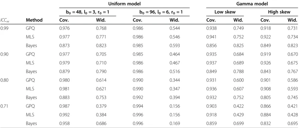
Table 3 Simulation study with uniform and gamma models

Uniform model Gamma model

b0= 48, l0= 3, r0= 1 b0= 96, l0= 6, r0= 1 Low skew High skew

ICCw Method Cov. Wid. Cov. Wid. Cov. Wid. Cov. Wid.

0.99 GPQ 0.976 0.768 0.986 0.544 0.938 0.749 0.918 0.731

MLS 0.977 0.771 0.986 0.546 0.941 0.752 0.922 0.734

Bayes 0.873 0.823 0.985 0.593 0.856 0.825 0.849 0.823

0.90 GPQ 0.977 0.705 0.985 0.464 0.935 0.684 0.919 0.670

MLS 0.979 0.710 0.986 0.467 0.937 0.689 0.926 0.675

Bayes 0.879 0.790 0.986 0.516 0.849 0.788 0.843 0.767

0.80 GPQ 0.980 0.614 0.990 0.344 0.931 0.600 0.901 0.586

MLS 0.981 0.621 0.990 0.347 0.936 0.607 0.908 0.593

Bayes 0.883 0.753 0.992 0.394 0.932 0.752 0.805 0.745

0.71 GPQ 0.987 0.379 0.994 0.156 0.903 0.422 0.866 0.421

MLS 0.992 0.384 0.996 0.156 0.918 0.429 0.884 0.428

Bayes 0.958 0.686 0.996 0.169 0.859 0.699 0.832 0.695

Comparison of MLS, GPQ and Bayes method performance on uniform and gamma data. Nominal 95% confidence intervals for ICCb. Coverages and average widths calculated from 10,000 simulations. In each case, ICCb= 0.70. Study designs have 48 biological replicates and 3 labs for a total of 144 observations, and 96 biological replicates and 6 labs for a total of 576 observations. Means and standard deviations of the point estimates of theICCbfor each setting are presented in

posterior distribution for the variance parameters is cal-culated, namely

f σ2

b;σ2l;σ2ejD

¼ f Djσ2b;σ2l;σ2e

π σ2

b;σ2l;σ2e

Z f Djσ2

b;σ2l;σ2e

π σ2

b;σ2l;σ2e

dσ2

bdσ2ldσ2e :

An explicit density formula will not generally exist. But Markov Chain Monte Carlo methods (e.g., Tierney [30]) can be used to generate a very large sample from this posterior distribution. Then, this sample can be used directly to estimate the posterior distribution of ρb= ICCb, that is, the densityf(ρb|D). The 95% credible

inter-val will contain area 0.95 under the posterior density curve. The highest posterior density (HPD) credible in-tervals will be the shortest possible credible interval [5] (p. 140).

Bayesian software have a variety of noninformative priors from which to choose. As discussed in the Additional file 1, we performed an extensive investigation of all the noninfor-mative priors on variance components that were offered, using as guidance advice in [6] and [35]. In the Results pre-sented in the paper, only the best performing noninforma-tive prior is shown. This turned out to be a uniform prior on the standard deviations, that is, the improper prior:

π σð b;σl;σeÞ ¼1 0ð <σb<∞Þ 1 0ð <σl<∞Þ

1 0ð <σe<∞Þ

The same prior was recommended by Gelman [35] (Section 7.1) for obtaining point estimates of individual variance parameters in a one-way analysis of variance, although in that context he warns that this prior can re-sult in miscalibration if the number of groups is small. In particular, the estimate of a variance component for a factor with a small number of levels will tend to be high.

Software

In this paper we developed our own programs for fre-quentist inference and these programs are available on-line at http://dobbinuga.com. The software SAS can also be used to construct MLS and GPQ intervals. Bayesian programs for constructing credible sets based on HPD regions include MCMCglmm [36] and winBUGS [33], among others. We use the MCMCglmm package to con-struct Bayesian HPD credible intervals. Implementation details are provided in the text. The simulation programs we wrote are available from the authors upon request.

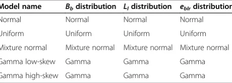
Simulation settings

In order to evaluate the different intervals, we looked at the performance metrics discussed above under the model assumption of Equation (1), and under violations of the model assumption. Simulations were run under

the settings in Table 4. Parameter values used are dis-cussed in Appendix C.

The value ofICCbwas examined at 0.7 and 0.9. These

represent reproducibility levels typically encountered in practice. When ICCb is 0.7, then the within-laboratory

(or within-rater, etc.) ICCw must be at least 0.70; we

ex-aminedICCw at 0.71, 0.80, 0.90, and 0.99, representing a

wide range of possible values. When ICCb= 0.9, we

ex-aminedICCw= 0.94.

The designs we examined had b0 as 48 or 96,

repre-senting moderate sized studies typically feasible for set-tings where resources are limited. The number of laboratories (or raters, etc.) used was 3 or 6, representing a setting where this number is restricted by logistics or costs.

Results Under normality

We first examine the different confidence interval methods when the effects and errors are normally distributed, so that the model assumptions are correct. Table 2 shows the results when there are 48 samples and 3 laboratories. The

ICCb= 0.70. Similar results were found for ICCb= 0.90

(Additional file 3). The coverage probabilities should be 95%. The GPQ method coverages are all within 0.01 of this target. All but one of the MLS coverages are within 0.01 of the target, with one setting being slightly conservative (coverage 0.968 whenICCw= 0.71). The coverage

probabil-ities of the Bayes intervals are below 95% in all cases, and below 90% in three of the four settings. The average width of each interval type decreases as theICCw decreases. In

all 4 settings, the widths of the MLS and GPQ intervals are practically identical. But in each setting the Bayes width is wider. This is surprising since wider intervals usually correspond to higher coverage. The excess width of the Bayesian intervals increases as the ICCw decreases, going

from 0.825-0.758 = 0.067 (Bayes width minus MLS width) up to 0.678-0.377 = 0.301 asICCwgoes from 0.99 down to

0.71.

Table 2 also shows the results when the number of la-boratories is doubled to 6 and the number of samples in-creases to 96. The coverage probabilities of the GPQ and MLS methods are within 0.01 of the 95% nominal

Table 4 Simulation settings

Model name _Bbdistribution Lldistribution eblrdistribution

Normal Normal Normal Normal

Uniform Uniform Uniform Uniform

Mixture normal Mixture normal Mixture normal Mixture normal

Gamma low-skew Gamma Gamma Gamma

Gamma high-skew Gamma Gamma Gamma

level in all cases. The Bayes methods are within 0.01 of the target in two of the four settings; in the other two settings, the Bayesian interval coverage is anticonserva-tive when ICCw= 0.99, and conservative when ICCw=

0.71 (coverages 0.930 and 0.964, respectively). The Bayesian method performance improves with the larger sample size and number of labs. In terms of interval widths, the GPQ and MLS methods are again indistin-guishable from one another. The Bayesian intervals are wider than the frequentist intervals in all scenarios.

Under violations of normality

We consider performance under model violations, that is, when neither the effects nor the errors are distributed according to the assumed normal distribution.

We first consider the uniform distribution. Table 3 shows the results with 48 biological replicates and 3 la-boratories. The GPQ and MLS methods both tend to have higher than nominal coverage, ranging from 0.976 to 0.992. The Bayesian method coverage is below 0.90 in three of the four settings, and is within 0.01 of the nominal in the other setting. The Bayesian methods only show minor improvement in coverage between the normal case and the uniform distribution case. As for interval width, the GPQ and MLS widths are again practically identical to one another throughout. The Bayesian widths are consist-ently larger. As was the case with the normal distribution setting, the Bayesian widths tend to both be wider and have lower coverage than the frequentist intervals.

When the number of biological replicates increases to 96 and the number of laboratories increases to 6 in the uniform model setting, the coverage probability for all methods increases (Table 3). In all cases, the coverage probability exceeds the nominal 95% level. The widths of the intervals are similar to those in Table 2 under the corresponding normal model. The Bayesian intervals are consistently wider than the frequentist intervals.

Table 3 also shows the results of comparison under the gamma model. The gamma distribution is intuitively a more serious violation of normality than the uniform distribution. When α = 3, the skewness is 1.15 (normal = 0) and the kurtosis is 5 (normal = 3). This is called the “high skew”model in the table (rightmost two columns). For the high skew setting, all methods have coverage probability below 93% across all scenarios. When ICCw

= 0.71, all methods have coverage below 90%. When the skewness and kurtosis are reduced (Table 3, “low skew” model with α =10 corresponding to skewness is 0.63 (normal = 0) the kurtosis is 3.6 (normal = 3)), the per-formance of all methods improve. Of note, the coverage probability of the frequentist methods are still below 92% when ICCw= 0.71. The Bayesian method has lower

coverage than the frequentist methods except for one case. Comparing the interval widths, the Bayesian

methods consistently have wider intervals than the fre-quentist methods across all of these settings. The two frequentist methods have very similar mean widths. Overall, while the frequentist methods appear slightly preferable to the Bayesian methods, none is ideal in the presence of skewed data.

Importantly, note that the departure from normality in the high skew gamma data is hard to detect in an actual fitted dataset. For example, we generated 10,000 datasets from the high skew gamma model. We fit the model to each dataset and performed the Shapiro-Wilk’s normal-ity test for the residuals. The mean p-value was 0.19, and the median was 0.08, and 55% of the p-values were above 0.05. For the low skew model, we did the same type of simulation and the mean Shapiro-Wilk’s residual p-value was 0.30 with a median of 0.20, and 69% of the p-values above 0.05.

A mixture normal distribution appeared similar to the normal distribution (Additional file 3).

Real data application: Barzman et al. study

This study involved 24 children (on video) rated by 10 different emergency room staff members. First, we followed the analysis described in Barzman et al. [15]. The analysis of variance table is shown in Table 5. If we represent the variance between the children by σ2_b; the variance between the staff members rating the videos by σ2

l;and the error variance byσ2e;then theICCbis σ

2 b

σ2 bþσ2lþσ2e:

The estimatedICCbreported in the paper is 0.9099. The

95% credible interval using noninformative priors re-ported in the Barzman et al. [15] paper is (0.8416, 0.9526). The 95% GCI that we computed with our pro-gram in this case is (0.8510, 0.9569). The Bayesian inter-val is about 5% wider than the GCI in this case, which is a trivial difference. The Bayesian interval is shifted to the left, relative to the frequentist interval, corresponding to lower estimates of the ICCb. But the shift is very minor,

and 96% of the GCI interval overlaps with the Bayesian interval, so that only 4% of the GCI interval does not overlap with the Bayesian interval.

Since we have discovered that the ICC intervals can be sensitive to violations of normality, we analyzed the data to assess normality of the effects and errors. First, we ana-lyzed transformations of the response variable using both the method of Box and Cox [37] and the modulus method [38]. Both methods indicated that the BRACHA scoresy

Table 5 ANOVA table from the Barzman et al. [15] study

Source DF SS MS

Raters 9 39.73 4.414

Children 23 2,195.35 95.450

should be transformed to approximately z= (y+ 0.5)0.55. Supporting the need for transformation, a test for regres-sion curvature had p-value 0.004, a Shapiro-Wilk test on the residuals had p-value 0.001, and a non-constant variance score test had p-value 0.001. On looking back at the raw data, it was observed that one child had one extreme outlying score. The child’s scores were (0,0,0,0,0,0,0,0,0.5,3.5). The one 3.5 is an extreme which had the largest Cook’s distance (0.11). Hence, a single rater’s unusual observation may be driving the apparent normality violation. To keep the model balanced, we therefore deleted this child’s data (child 11), resulting in 23 children. Re-analyzing the data from scratch resulted in the same transformation of the BRACHA scores. How-ever, the regression test for curvature had p-value of 0.43, the Shapiro-Wilk normality test on the residuals had p-value 0.51, and the non-constant variance score test had p-value 0.19. Thus, there is no longer any evidence of lack of normality. The mean squares were 8.3721, 0.3667, 0.0671 for the reduced dataset. The resulting 95% gene-ralized confidence interval for ICCb is (0.8423, 0.9542).

Although it did not have a large impact on the confidence interval in this case, the process outlined here of carefully assessing normality and revising the analysis as needed, should be part of interval construction. The reason for the minor impact on the interval in this case, compared to the simulations, may be the large number of raters (10 raters).

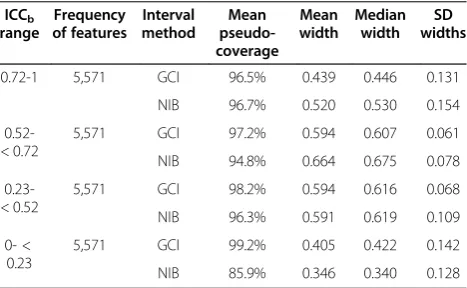
Real data application: NCI DC reproducibility study The National Cancer Institute’s Director’s Challenge repro-ducibility study examined the reprorepro-ducibility of 22,283 fea-tures represented on the Affymetrix U133A Genechip across a collection of frozen patient tissue samples. Unlike other technologies that measure the level of a single gene at a time, microarrays measure the levels of expressions of thousands of human genes simultaneously. The expression measurements are continuous, so that for each individual gene one can assess the reproducibility of the measure-ments for that particular gene across the different samples by calculating theICCb. The result is 22,283 different

re-producibility estimates, one for each feature. The NCI DC reproducibility study was one of the largest studies of the reproducibility of microarrays, and thus is of interest in terms of the strength of the conclusions we can draw. To this end, we constructed confidence intervals for all 22,283 features using both the frequentist and Bayesian ap-proaches. For the confidence interval constructions, some samples were omitted to force the design to balance. The result was 4 labs and 11 samples for a total of 44 observa-tions for each feature. Data were normalized as in Dobbin et al. [16] except that dChip [39] was used instead of MAS 5.0 (http://www.affymetrix.com/support/technical/ whitepapers.affx). We first applied both Bayesian and

frequentist methods to construct confidence intervals for each feature. Results are shown in Table 6. For features with reasonably high reproducibility (ICCb> 0.52, top 2

quartiles of features) the interval widths for the GCI’s had lower mean and median than the corresponding Bayesian interval widths.

In order to estimate the coverage probabilities of the DC reproducibility study intervals, we considered the 44 samples examined as a random sample from a finite popu-lation which consisted of all 69 tumor microarrays in the original dataset. For this “population” of 69 samples, the true ICCb values were calculated from the unbalanced

data, using the expected mean squares presented in [16]; we can call these values pseudo-parameters, to distinguish them from the true population parameters, which are un-known. The proportion of times the pseudo-parameters were contained in each interval was calculated; we term this pseudo-coverage. Note that pseudo-coverage is equal to the true coverage for the finite population of 69 sam-ples. As shown in Table 6, for features with ICCb> 0.72,

representing the quartile with the highest reproducibility (highest pseudo-parameter values), the pseudo-coverage of the frequentist and Bayesian methods are similar (96.5% and 96.7%, respectively), but the GCI interval width mean is much smaller than the NIB interval width mean (0.439 versus 0.520, or 16% narrower GCI). These width differ-ences are similar to those observed in the simulations. Interestingly, Table 6 also reveals that the NIB coverage breaks down (with coverage only 85.9%) when ICCb≤

0.23, while the GCI maintains high coverage (with cover-age 99.2%) in this setting. This observation suggests that the Bayesian methods may undercover when the point es-timate of theICCbis small.

Because of the importance of normality of the data, we re-evaluated the DC reproducibility study more closely with this in mind. First we performed the method of Box and Cox [37] for the linear model of Equation 1 for

Table 6 DC lung study results

ICCb range

Frequency of features

Interval method

Mean pseudo-coverage

Mean width

Median width

SD widths

0.72-1 5,571 GCI 96.5% 0.439 0.446 0.131

NIB 96.7% 0.520 0.530 0.154

0.52-< 0.72

5,571 GCI 97.2% 0.594 0.607 0.061

NIB 94.8% 0.664 0.675 0.078

0.23-< 0.52

5,571 GCI 98.2% 0.594 0.616 0.068

NIB 96.3% 0.591 0.619 0.109

0- < 0.23

5,571 GCI 99.2% 0.405 0.422 0.142

NIB 85.9% 0.346 0.340 0.128

each gene to assess the optimal normalizing transform-ation. The distribution of the Box-Cox lambda values is shown in the Additional file 1. There is some variation in the estimated optimal lambda values. They are cen-tered near zero. Zero corresponds to the log transform-ation used in the previous analysis for all features. However, since normality is so important for ICC inter-val inter-validity, we re-analyzed these data using the gene-specific Box-Cox transformations. We ran the Tukey interaction tests on all features, and all had p-values over 0.05, indicating no evidence of interaction effects. The resulting Shapiro Wilk test p-value distribution had mean of 0.44, and approximately 12% of features had a p-value below 0.05. There appeared to be no patterns in the Shapiro Wilk p-values that would be useful in identi-fying the normally distributed genes. Our conclusion is that the confidence intervals for most features should be valid, but that individual feature CI’s should be inter-preted in the context of the corresponding Shapiro Wilk test p-value.

Discussion

Two questions arise from these observations. (1) Why are the noninformative Bayesian methods performing poorly relative to the frequentist methods in some cases? (2) Why are both methods not robust to skewness and kurtosis?

For question 1, these results naturally led us to further investigate the Bayesian credible interval methodologies. When the Bayesian and frequentist intervals differed, the midpoints of the Bayesian intervals tended to be further from the trueICCbthan the midpoints of the frequentist

intervals. The result we saw was wider intervals with poorer coverage. But why did this happen? Detailed dis-cussion appears in the Additional file 1. In summary, we discovered potential reasons for the poor performance of the noninformative Bayesian priors. One issue is that

noninformative priors on variance components do not imply noninformative distributions on the ICC. In fact, we derive these distributions in the Additional file 1 and show that they can be nearly point masses at 0 and 1. The one distribution where this is not the case is the one that works best in practice, namely, the uniform distribution on the standard deviation. But even this prior distribution on theICCbhas most of its mass towards the edges of the

unit interval (Additional file 1: Figure S2). That being said, this fact probably does not entirely explain the poor per-formance. The second potential issue is thatthe Bayesian methods are not based on an underlying exact interval construction method, like the GCI and the MLS methods. Put another way, the modified large sample method uses a “modified” version of the usual large sample method, whereas the Bayesian methods use an “ un-modified” Bayesian computation. Indeed, since the GCI

method is closely related to the nonparametric Bayesian method [34], it may be that nonparametric Bayesian methods can be used to adjust the Bayesian parametric intervals.

The lack of robustness to skewness and kurtosis may ap-pear surprising given that analysis of variance in general is robust to these. However, since we are constructing a con-fidence interval for a ratio of variance components, this means that estimation becomes more unstable. For ex-ample, the MLS interval equation involves fourth order moments. In general, the higher order a moment is, the more difficult it is to estimate. The GCI method, while not relying explicitly on fourth order moments, relies on the assumption that the second order moments are chi-squared in order to estimate quantiles of the generalized pivot, which is conceptually quite similar to calculating a fourth order moment.

Conclusions

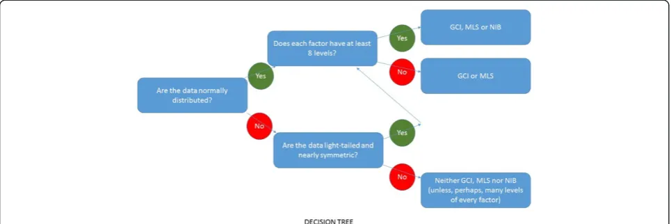
In this paper several methods for constructing intervals for the intraclass correlation coefficient were examined. Coverage probabilities and confidence interval widths were reported for the commonly encountered two-way, crossed-effects linear model without interaction. The Modified Large Sample (MLS), Generalized Confidence Interval (GCI) and noninformative Bayesian interval methods were evaluated. When model assumptions are true, we showed that the MLS and GCI methods perform well under a wide range of settings. Bayesian software with noninformative priors on variance components did not perform as well in most settings, often failing to achieve desired coverage and at the same time, counterintuitively, also resulting in wider average interval widths. Under model violations, it was shown that the methods performed similarly when there was small skewness and kurtosis. However, neither the fre-quentist nor the Bayesian methods were robust to hard-to-detect skewness and kurtosis when the number of levels of one factor is small. The methods were applied to two previ-ously published reproducibility studies and new insights were gained. Future directions to improve the Bayesian ap-proaches were suggested. A decision tree summarizing this paper’s findings is presented in Figure 1.

coefficient (either ICCbor ICCw). Moreover, this change

is a function of the user-defined choice of non-informative prior parameter, so that IG(0.001,0.001) pro-duces very different intervals than IG(0.01,0.01); a simi-lar result was reported by Gelman [35] in the context of making inference about individual variance components. The uniform prior used in this paper does not result in a nearly degenerate prior for the ICC, is not affected by scale changes in the data, and is not sensitive to user-defined parameter choices (trivially, since there are none).

A question outside the scope of this paper is whether it is possible to develop Bayesian methods that would have performance comparable to the frequentist methods across all scenarios in terms of mean interval width and coverage probability. It is possible that at some point in the future such a method will be developed. One possibil-ity mentioned in the discussion is adapting nonparametric Bayesian methods for random effects models to this set-ting (for discussion, see [40]). Another possibility, follow-ing a suggestion in Gelman [35], is to have a relatively minor modification of the prior and place uniform distri-butions on individual variance components with finite support, so thatσ~Uniform(0,k) for somek> 0; a differ-ent constant k could be used for each variance compo-nent, and these would need to be chosen based on prior knowledge or on the data (e.g., empirical Bayes). Indeed, the utility of Bayesian methods in medical contexts where prior or expert knowledge is available is widely recognized. Further research in this direction seems needed.

In modeling laboratory reproducibility, we have assumed that the effect of a laboratory is represented by a tendency to score higher or lower than other laboratories across bio-logical samples assayed. But laboratory effects may be rep-resented in other ways. For example, it may be that some laboratories have higher variance in their measurements, but no systematic difference across individuals. Such a

setting could be represented by a variance components model that allowed each lab to have its own within-laboratory measurement error variance (that is, in Equation (1), permitσ2_e to vary by laboratory). This would represent that lab’s ability to obtain replicable measurements in re-peated assays. The null hypothesis that all within-lab variances are equal could be tested against the general alternative. Alternatively, the CCC could be used [18], as suggested by a referee. As another example, an inter-action between labs and samples could be introduced into Equation 1 to represent lab-to-lab variation in ability to re-producibly measure individual samples, and indeed we have used a Tukey test to assess such interaction in the first application.

We used simulation to investigate whether we could de-velop post-hoc rules which could be used to select an inter-val construction method. Unlike Figure 1, these rules would be based on the values of the observed mean squares, in addition to the study design and normality as-sumptions. We were unable to come up with helpful rules that could be used in practice. But these results (not pre-sented) suggested that the Bayesian methods tend to underperform more often when the laboratory variance es-timate is large relative to the biological variance, and that the frequentist tend to underperform when the estimated biological variance is very large relative to the estimated la-boratory variance. But we discourage investigators from using these broad observations in selecting a methodology, and recommend instead Figure 1.

Bayesian, MLS and GCI would all be very similar and ad-equate under the normal model assumptions. The Bayesian coverages are similar to the frequentist for even 4-6 levels, but the Bayesian interval widths are noticeably wider.

Appendix A: formula for the generalized pivotal quantity

G¼ max 0;c2s 2

b=W2−c3s2e=W3

c1s2l=W1þc2sb2=W2þc4s2e=W3

where c2= (b0−1)/(l0r0),c3= (b0l0r0−b0−l0+ 1)/(l0r0),

c1= (l0−1)/(b0r0) and c4=c3(b0l0r0−b0−l0+ 1)/b0. Here

W1eχ2ð_l0−1Þ W2eχ2ð_b0−1Þ and W3eχð2_{b0l0r0−b0−l0}þ1Þ are mutu-ally independent given the observed mean squares. Gen-erating a large number of (W1,W2,W3) triples (such as

100,000) by Monte Carlo, the generalized confidence interval is formed from the quantile functionF^−_G1:

Appendix B: modified large sample formula The formula for the interval (L,U) is

L¼ max 0;L

f g

1þ max 0f ;Lg;U¼

max 0f ;Ug 1þ max 0f ;Ug

L¼b0ð1−G2Þs 2

b−b0s2bs2eþb0 F5−ð1−G2ÞF25

s2

e l0ðb0r0−1Þs2bs2eþl0ð1−G2Þs2bs2l=F4

U¼b0ð1þH2Þs 2

b−b0s2bs2eþb0 F6−ð1þH2ÞF26

s2_e l0ðb0r0−1Þs2bs2eþl0ð1þH2Þs2bs2l=F3

where the constants G2,F5,F4,H2,F6,F3 are quantiles

of F distributions as defined in the Additional file 1 and [25].

Appendix C: simulation parameter settings

Additional file 1: Table S1 shows the complete list of simulation settings used. Simulation results not pre-sented in the paper appear in the Additional file 3. For the simulations involving the normal distribution, data were generated as given in Equation 1 above.

The robustness of intervals to violations of the nor-mality assumption was evaluated by generating effects and errors from uniform, mixture normal, and gamma distributions. Parameters settings were calculated to make the variances of the simulated biological effects, lab effects and measurement error exactly the same as in the normal simulations.

For a random variable X with the uniform distribution on the interval [-A,A], the variance is Var(X) =A2/3. This leads to the formulas

Ab¼ ffiffiffiffiffiffiffiffi 3σ2

b q

;Al¼ ffiffiffiffiffiffiffiffi 3σ2

l q

;Ae ¼ ffiffiffiffiffiffiffiffi 3σ2

e q

If the distribution of each effect in Equation (1) is uni-form, instead of normal, then the marginal distribution of

the responses, Yblr, are sums of uniform random variables.

The marginal density is derived in Additional file 1: Sec-tion S5 and plotted in the AddiSec-tional file 1.

A random variable X with a normal mixture distribu-tion with means ±μ and standard deviations μ/3, and weights 0.5, will be bimodal. We can write the mixture normal as a hierarchical model with c ~ Bernoulli(0.5), and

X_e Normalðμ;μ2=9Þ :c¼0 Normalð−μ;μ2=9Þ :c¼1

Then E[X] = 0 and Var(X) =μ2*(10/9).

The resulting equations are μ_b¼ ffiffiffiffiffiffiffiffiffiffiffiffiffiffiffi9σ2

b=10 p

;μl¼ ffiffiffiffiffiffiffiffiffiffiffiffiffiffiffi

9σ2

l=10 q

;μe¼

ffiffiffiffiffiffiffiffiffiffiffiffiffiffiffi

9σ2

e=10 p

: The marginal densities for Yblrare also mixture normal (see Additional file 1: Section

S5), and are shown in the Additional file 1.

Define Gamma(α,β) by the density function f xð Þ ¼

1

Γ αð Þβαxα−1e−x=β: Effect sizes and errors are generated by the following steps:

w0eGammaðα;1Þ w1¼w0−α w¼ðσ=pffiffiffiαÞw1

Note that w can be viewed as a mean-shifted version of w0 σ= ffiffiffiα

p

ð Þ; and since central moments are

translation-invariant, the central moments of w are the same as the central moments of a Gamma(α,σ/α1/2). As a result, E[w] = 0, Var(w) =σ2, skewness(w) = 2=pffiffiffiαand kurtosis(w) = 3 + 6/α[41] (p. 31). We keep β= 1. We let

α = 1, 3, 10, 40. The marginal densities forYblr are

dis-cussed in Additional file 1: Section S5 and shown in the Additional file 1.

Additional files

Additional file 1:Supplement includes additional discussion, simulations, data analysis details, figures and tables.

Additional file 2:Supplement presents the mean and standard deviation of the point estimates of the ICCb for different models and designs presented in the main paper.

Additional file 3:Supplement presents complete tables of the core simulations simulations from which the tables in the paper are a subset.

Additional file 4:Supplement is a table of results for designs with 8, 10, 12, 14 and 16 factor levels for laboratories.

Additional file 5:Supplement is a table of results for designs with 4, 5, 6 and 7 factor levels for laboratories.

Competing interests

The authors declare that they have no competing interests.

Authors’contributions

development and writing. All authors read and approved the final manuscript.

Acknowledgments

Ionan and Dobbin were supported in part by a grant from the Georgia Research Alliance’s Distinguished Cancer Scholars Program.

Author details 1

Department of Statistics, University of Georgia, Athens, GA, USA.2Biometric Research Branch, National Cancer Institute, Rockville, MD, USA.3_Department

of Epidemiology and Biostatistics, University of Georgia, Athens, GA, USA.

Received: 6 May 2014 Accepted: 27 October 2014 Published: 22 November 2014

References

1. Bartko J:Intraclass correlation coefficient as a measure of reliability.

Psychol Rep1966,19:3–11.

2. Donner A:The use of correlation and regression in the analysis of family resemblance.Am J Epidemiol1979,110(3):335–342.

3. Wolak M, Fairbairn D, Paulsen Y:Guidelines for estimating repeatability.

Methods Ecol Evol2012,3(1):129–137.

4. Gisev N, Bell J, Chen T:Interrate agreement and interrater reliability: key concepts, approaches, and applications.Res Soc Admin Pharm2013,

9(3):330–338.

5. Berger J:Statistical Decision Theory and Bayesian Analysis.2nd edition. New York: Springer-Verlag; 1985.

6. Carlin B, Louis T:Bayesian Methods for Data Analysis.3rd edition. Boca Raton, FL: Chapman and Hall; 2009.

7. Little R:Calibrated Bayes: a Bayes/frequentist roadmap.Am Stat2006,

60:213–223.

8. Rubin D:Bayesianly justifiable and relevant frequency calculations for applied statisticians.Ann Stat1984,12:1151–1172.

9. Box G:Sampling and Bayes inference in scientific modeling and robustness.J Royal Stat Soc A1980,143:383_–430.

10. Browne W, Draper D:A comparison of Bayesian and likelihood-based methods for fitting multilevel models.Bayesian Anal2006,1(3):473–514. 11. Yin G:Bayesian generalized method of moments.Bayesian Anal2009,

4:191–208.

12. Leonard D:Estimating a bivariate linear relationship.Bayesian Anal2011,

6:727–754.

13. Bingham M, Vardeman S, Nordman D:Bayes one-sample and one-way random effects analyses for 3-D orientations with application to materials science.Bayesian Anal2009,4:607_–630.

14. Samaniego F:A Comparison of the Bayesian and Frequentist Approaches to Estimation.New York: Springer; 2010.

15. Barzman D, Mossman D, Sonnier L, Sorter M:Brief rating of aggression by children and adolescents (BRACHA): a reliability study.J Am Acad Psychiatry Law2012,40:374_–382.

16. Dobbin K, Beer D, Meyerson M, Yeatman T, Gerald W, Jacobson J, Conley B, Buetow K, Heiskanen M, Simon RM, Minna JD, Girard L, Misek DE, Taylor JM, Hanash S, Naoki K, Hayes DN, Ladd-Acosta C, Enkemann SA, Viale A, Giordano TJ:

Interlaboratory comparability study of cancer gene expression analysis using oligonucleotide microarrays.Clin Cancer Res2005,11:565–572.

17. McShane LM, Aamodt R, Cordon-Cardo C, Cote R, Faraggi D, Fradet Y, Grossman HB, Peng A, Taube SE, Waldman FM:Reproducibility of p53 immunohistochemistry in bladder tumors. National cancer institute, bladder tumor marker network.Clin Cancer Res2000,6(5):1854–1864. 18. Chen C, Barnhart HX:Comparison of ICC and CCC for assessing

agreement for data without and with replications.Comput Stat Data Anal

2008,53:554–564.

19. Lin LI, Hedayat AS, Wu WM:Statistical Tools for Measuring Agreement.New York: Springer; 2012.

20. Montgomery D:Design and Analysis of Experiments.8th edition. New York: Wiley; 2013.

21. Searle S, Fawcett R:Expected mean squares in variance components models having finite populations.Biometrics1970,26(2):243–254. 22. Lin LI, Hedayat AS, Wu WM:A unified approach for assessing agreement

for continuous and categorical data.Biopharm Stat2007,17(4):629–652.

23. Cappelleri J, Ting N:A modified large-sample approach to approximate interval estimation for a particular class of intraclass correlation coefficient.Stat Med2003,22:1861–1877.

24. Graybill F, Wang C:Confidence intervals for nonnegative linear combinations of variances.J Am Stat Assoc1980,75:869–873. 25. Burdick R, Borror C, Montgomery D:Design and Analysis of Gauge R&R

Studies: Making Decisions with Confidence Intervals in Random and Mixed ANOVA Models.Alexandria, Virginia: ASA and SIAM; 2005.

26. Arteaga C, Jeyaratnam S, Graybill F:Confidence intervals for proportions of total variance in the two-way cross component of variance model.

Commun Stat Theor Methods1982,11:1643–1658.

27. Weerahandi S:Generalized confidence intervals.J Am Stat Assoc1993,

88(423):899–905.

28. Robert C, Casella G:Monte Carlo Statistical Methods.New York: Springer; 2010.

29. Gelfand A, Smith A:Sampling based approaches to calculating marginal densities.J Am Stat Assoc1990,85:398–409.

30. Tierney L:Markov chains for exploring posterior distributions.Ann Stat

1991,22:1701–1762.

31. Metropolis N, Rosenbluth A, Rosenbluth M, Teller A, Teller E:Equations of state calculations by fast computing machines.J Chem Phys1953,

21:1087–1092.

32. Thomas A, O’Hara B, Ligges U, Sturtz S:Making BUGS open.R News2006,

6:12–17.

33. Lunn D, Thomas A, Best N:WinBUGS–a Bayesian modeling framework: concepts, structure and extensibility.Stat Comput2000,10:325–337. 34. Weerahandi S:Exact Statistical Methods for Data Analysis.New York:

Springer-Verlag; 2003.

35. Gelman A:Prior distributions for variance parameters in hierarchical models.Bayesian Anal2006,1(3):515–533.

36. Hadfield J:MCMC methods for multi-response generalized linear mixed models: the MCMCglmm R package.J Stat Software2010,33(2):1–22. 37. Box G, Cox D:An analysis of transformations (with discussion).J Royal

Stat Soc B1964,26:211–252.

38. John J, Draper N:An alternative family of transformations.Appl Stat1980,

29:190–197.

39. Li C, Wing WH:Model-based analysis of oligonucleotide arrays: expression index computation and outlier detection.Proc Natl Acad Sci U S A2001,98(1):31–36.

40. Muller P, Quintana F:Nonparametric Bayesian data analysis.Statistical Science2004,19(1):95–110.

41. Lehman E, Cassella G:Theory of Point Estimation.New York: Springer; 1998.

doi:10.1186/1471-2288-14-121

Cite this article as:Ionanet al.:Comparison of confidence interval methods for an intra-class correlation coefficient (ICC).BMC Medical Research Methodology201414:121.

Submit your next manuscript to BioMed Central and take full advantage of:

• Convenient online submission

• Thorough peer review

• No space constraints or color figure charges

• Immediate publication on acceptance

• Inclusion in PubMed, CAS, Scopus and Google Scholar

• Research which is freely available for redistribution