Path Planning and Obstacle Avoidance for Boe Bot Mobile Robot
Mohamed Ghorbel1, Lobna Amouri1, Christian Akortia Hie2 1Institute of Electronics and Communication of Sfax (ISECS) ATMS-ENIS,University of Sfax
BBP 1173, 3038, Tunisia
2Private Polytechnic Institute of Sfax University of Sfax, Tunisia
ABSTRACT: This paper focus on the control problem of unicycle mobile robot using regular approach. The potential field method is used to ensure robot navigation while avoiding obstacles present in the surrounding environment. Simulation and experimental tests are carried out on a “Boe Bot” mobile robot and proved the effectiveness of the studied method.
Keywords: Mobile robots, Robot Navigation
Received: 12 November 2012, Revised 24 December 2012, Accepted 29 December 2012
© 2013 DLINE. All rights reserved
1. Introduction
Many researches have investigated, during the last decades, the guidance of land autonomous vehicles, underseas robots, manipulators and walking machines. Many experiments have been carried out on real robots (wheeled mobile robots, and AUV) and on simulated ones [6], [3]. A real-time obstacle avoidance algorithm coupled with path following is studied and implemented in this paper.
In recent years, much interest has been focused upon the new numerical control strategies (PID) who’s performances are compromised by large variations in the state space, and by parameter variations. Robust nonconventional control strategies called fuzzy logic are also used in the area of process control [5], [7]. In fact, these methods are generally used to deal with nonlinear sytems [4].
The most famous reacted approach is the potential method developed by O.Khatib [1]. It consists in building an arbitrary positive potential field functions attached on obstacles that repels the robot and an attractive field located on the target. This technique was been ameliorated by Borenstein researches [2] through mading a vector field histogram attached on proximity information.
In this paper we studied a regular approach computed with the potential method in the case of a mobile robot by underlying two different parts:
• The control
The obstacle detection is an important topic and in this paper we have considered a mobile robot equipped with infra-red sensors able to measure the distance between the robot and its environment. This paper is organized into five sections. In section 2 the model of the robot and its equipments are presented. In section 3 the mathematical formulation for pathfollowing and obstacle avoidance is described. Finally, section 5 contains the results of the simulation and experimental tests.
2. Robot Equipment
The robot Boe Bot is a unicycle robot with one steering wheel and two independent driving wheels, which can be oriented and commanded by acting on the speed of each wheel, as shown on the schematic model (Figure 1).
Figure 1. The schematic model of a wheelchair The kinematic model is given by:
dXR
dYR
VR + VL
L
2
dθR dt
dt
dt
VR + VL
2
VR − VL =
=
= cosθR
sinθR
⎩
⎨
⎧
where VR and VL are the robot’s right and left wheel’s velocities, respectively; θR is the robot’s angular velocity, L is the distance between two wheels and R is the angle between the robot’s direction and the X-axis. By discretization of the system (1) using Euler method, it becomes:
XRnew = XRold + T
YRnew = YRold + T
θRnew = θRold + T
VR + VL
2 cosθR old old
old
VR + VL
2 sinθR old old old
pulses = d
speedtemp
temp = lr + ll + Texe + T
⎩ ⎨ ⎧
with: lr (ms) and lr (ms) are the impulses width respectively for the right and left wheels. Texe is an instruction run time.
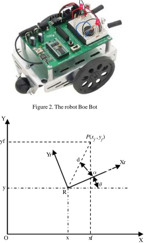
The robot is provided with an infra-red senor. The infra-red transmitter is QEC113 while the receiver is PNA4602M. The following figure (Figure 2) presents the robot with its equipments.
Figure 2. The robot Boe Bot
(3) where T is the sampling time. The robot displacement is function of its two servomotors controlling the two driving wheels. The command is made by series of periodic impulses. The impulse width noted L presents the angular position to be achieved by servomotors. In order to generate the accurate number of pulses number needed to achieve an arbitrarydistance noted d, we have used the following equations:
3. Mathematical Formulation
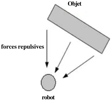
This section presents the mathematical formulation either for the path following and the obstacle avoidance algorithms. Figure 3. Robot polar coordinates
O x xf X
y yf Y
Yr
R
Xr d
θ α
3.1 The path following method
In order to ensure the robot autonomy during its navigation in different paths, we have to generate the robot polar coordinates. Figure 3 described the polar coordinates between the robot and a desired point in the path.
These coordinates provide the correction of the angular velocity (w) and the linear velocity (ν) as shown in the following equation system.
α = arctan yf
xf
⎝ ⎛
⎠ ⎞− θ
v = k1 d cosα
w = k2α + k1 sinαcosα
⎩
⎨
⎧
With k1 and k2 are constants calculated basing on simulation and experimental tests.
3.2 The obstacle avoidance method
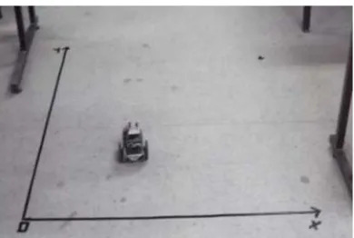
The obstacle avoidance strategy we used is the potential field method. Its principle consists in generating two potential fields. The first one is functions field attached on obstacles that repels the robot. The second field is an attractive one located on the target. Figure 4 showed the principle of this method The path following controller described in the previous section was been,consequently, so that the robot succeeded to avoid the present obstacle while reaching the path. The obtained new sytem equation is presented as follows:
Figure 4. Repulsive fields
dr = fr2 + d 2
β = arctan fr
dr
⎝ ⎛
⎠ ⎞
ν = k1 dr cosβ
w = k2β + k1 sinβ cosβ
⎩
⎨
⎧
(4)
(5) forces repulsives
robot
Objet
With: dr is the resultant distance between the robot and an obstacle. fr is a repulsive force.
4. Results
Initially, the simulation tests were carried out with the Matlab software. We have choosed fr = 100cm and d = 5cm. While experimental were carried out with the Basic Stamp software. The navigation environment is a square platform as shown in the following figure 5.
Figure 5. Experimental environment
Figure 6. simulation result with k1 = 1 and k2 = 10
Figure 7. Simulation result with k1 = 10 and k2 = 0 -25 0 25 50 75 100 125 125
100
75
50
25
0
-25
axe des X (en cm)
axe des Y (en cm)
125
100
75
50
25
0
-25
-25 0 25 50 75 100 125
axe des X (en cm)
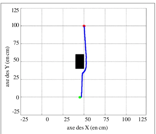
Figure 8. Path following and obstacle avoidance
Figure 9. Step 1 Figure 10. Step 2 Figure 11. Step 3
Figure 12. Step 4 Figure 13. Step 5 Figure 14. Step 6
Figure 15. Step 7 Figure 16. Step 8 Figure 17. Step 9 -25 0 25 50 75 100 125
axe des X (en cm)
axe des Y (en cm)
125
100
75
50
25
0
Figures 6 and 7 showed that the robot reached the desired target in both cases. But, the obtained curves demontrate the influence of the parameter k2 in optmizing the trajectory.
• Simulation 2: The purpose of the second simulation is to show the effectiveness of the computation between the path following and obtacle avoidance. The trial showed the success of the adopted trategy.
• Experimental result: The obstacle avoidance method computed with path following is finally implemented on the robot base. During this course (figure 9.. figure 17) we noticed that the robot avoid the obstacle and attempts the final target.
5. Conclusion
We have designed an obstacle avoidance control for a mobile robot based on the potential field approach. The implementation of the algorithm demonstrate the effectiveness of the proposed method in order to avoid some obstacles. In this way, we control the robot despite his inertia and response time. To further improve the obtained results we propose to combine reactive behaviours with some local methods (as fuzzy logic).
References
[1] Kathib, O. (1985). Real-Time Obstacle Avoidance for Manipulators and Mobile Robots. In:Proc. IEEE Inernational Conference on Robotic and Automation(ICRA 1985), p. 500-505.
[2] Borenstein, J., Koren, Y. (1991). The Vector Field Histogram-Fast Obstacle avoidance for Mobile Robots. IEEE Transactions on Robotics and Automation, 7 (3) 278-288, June.
[3] Elnagar, A., Hussein, A. (2002). Motion Planning using Maxwell’s quations. IEEE International Conference On Intelligent Robots and Systems, Lausanne, Switzerland, October.
[4] Minguez, J., Montano, L., Santos-Victor, J. (2002). Reactive navigation for nonholonomic robots using the ego-kinematic space. International Conference on Robotics and Automation (ICRA 2002). USA, Mai.
[5] Amouri-Jmaiel, L., Jallouli, M., Derbel, N. (2009). An Effective Sensor Data Fusion Method for Robot Navigation Through Combined Extended Kalman Filters and Adaptive Fuzzy Logic, Transactions on Systems, Signals and Devices TSSD, 4 (1) 1-18. [6] Njah, M., Jallouli, M., Derbel, N. (2009). A Synthesis of a fuzzy controller for the navigation of an electric wheelchair for handicapped persons, Multi-conference on Signals Systems and Devices (SSD 2009), Djerba, Tunisia.