Second-order differential equations with deviating arguments

DEVIATING ARGUMENTS

Received 2 May 2006; Revised 22 May 2006; Accepted 28 May 2006

This paper deals with boundary value problems for second-order differential equations with deviating arguments. Some sufficient conditions are formulated under which such problems have quasisolutions or a unique solution. A monotone iterative method is used. Examples with numerical results are added to illustrate the results obtained.

Copyright © 2006 T. Jankowski and W. Szatanik. This is an open access article distributed under the Creative Commons Attribution License, which permits unrestricted use, dis-tribution, and reproduction in any medium, provided the original work is properly cited.

1. Introduction

Let us consider a problem

x(t)=ft,x(t),xα(t)≡Fx(t), t∈J=[0,T],T <∞,

x(0)=0, x(T)=rx(γ) withγ∈(0,T), (1.1)

where f ∈C(J×R×R,R) andα∈C(J,J) (e.g.,αmay be defined byα(t)=√t,T≥1 or α(t)=0.7t,t∈J). Moreover,randγare fixed real numbers.

Differential equations with deviated arguments arise in a variety of areas of biologi-cal, physibiologi-cal, and engineering applications, see, for example, [9, Chapter 2]. The mono-tone iterative method is useful to obtain approximate solutions of nonlinear differential equations, for details see, for example, [10], see also [1–8,11,12]. It has been applied successfully to obtain results of existence of quasisolutions for problems of type (1.1), see [4]. In paper [4], it was assumed that functionf satisfies a one-sided Lipschitz condition with respect to the last two variables with corresponding functions instead of constants. Note that the special case whenf is monotone nonincreasing (with respect to the last two variables) is not discussed in paper [4] and is of particular interest. Moreover, at the end of this paper we formulate conditions under which problem (1.1) has a unique solution. This paper extends some results of [4].

Hindawi Publishing Corporation Boundary Value Problems

The plan of this paper is as follows. InSection 3, we discuss problem (1.1) for the case whenr≤0.Theorem 3.1says about extremal quasisolutions of problem (1.1).Example 3.2illustrates that assumptions ofTheorem 3.1are satisfied, so the problem (3.13), from this example, has extremal quasisolutions which are the limit of sequences{yn,zn}. To

obtain an approximate extremal quasisolutions we can use the elements of sequences

{yn,zn}.Using numerical methods we can find numerical approximationsyn,znofyn,zn,

respectively. The graphs of someyn,znare given inFigure 3.1. InSection 4, we investigate

problems having more deviating arguments. Also an example and graphs of numerical approximations ofyn,znare given. InSection 6, we combined results of this paper with

corresponding results of [4].Example 6.5shows the results obtained. In the last section, we investigate the problem when the minimal and maximal quasisolutions are equal, so when our problem has a unique solution.

2. Lemmas and definitions

We need some lemmas which are useful in this paper. It is easy to show the following.

Lemma2.1. Letp∈C2_(J,R)and

p(t)≥0 fort∈J,

p(0)≤0, p(T)≤0. (2.1)

Thenp(t)≤0onJ.

It is a well-known fact which follows from Green function properties that the following holds.

Lemma2.2. Let

G(t,s)= −1

T ⎧ ⎪ ⎨ ⎪ ⎩

(T−t)s for0≤s≤t≤T, (T−s)t for0≤t≤s≤T.

(2.2)

Leth:J→Rbe integrable onJ. Then the problem

u(t)=h(t), u(0)=0, u(T)=β (2.3)

has exactly one solution given by

u(t)=

T

0 G(t,s)h(s)ds+ β

Tt. (2.4)

Definition 2.3. A pair of functions y0,z0∈C2(J,R) is calledcoupled lower and upper solutions of (1.1) if

y0(t)≥Fz0(t), y0(0)≤0, y0(T)≤rz0(γ),

z0(t)≤F y0(t), z0(0)≥0, z0(T)≥r y0(γ),

(2.5)

wheret∈J.

Definition 2.4. A pair of functionsY,Z∈C2_{(J,R) is calledcoupled quasisolutionsof (1.1)} if

Y(t)=FZ(t), Y(0)=0, Y(T)=rZ(γ),

Z(t)=FY(t), Z(0)=0, Z(T)=rY(γ), (2.6)

wheret∈J.

Let f,g∈C2_{(J,R) and f(t)≤g(t) fort∈J. We will say that a functione∈C}2_(J,R) belongs to segment [f,g] if f(t)≤e(t)≤g(t) fort∈J.

Definition 2.5. Let a pair (U,V) be a coupled quasisolutions of (1.1). (U,V) are called minimal and maximal coupled quasisolutionsof (1.1) if for any elseU,V coupled qua-sisolutions of (1.1), it holds thatU(t)≤U(t),V(t)≤V(t),t∈J.

Letu,v∈C2_{(J,R) satisfyu(t)≤v(t) fort∈J. Coupled quasisolutionsU,V of (1.1)} are calledminimal and maximal coupled quasisolutionsin segment [u,v] ifu(t)≤U(t), V(t)≤v(t) fort∈Jand for any else (Y,Z) coupled quasisolutions of (1.1), such asu(t)≤

Y(t),Z(t)≤v(t) fort∈J, it holds thatU(t)≤Y(t) andZ(t)≤V(t),t∈J.

Remark 2.6. Note that if a function yis a solution of (1.1), then the pair (y,y) will be coupled quasisolutions of (1.1).

3. Main results ifr≤0

Now we formulate conditions which guarantee that problem (1.1) has extremal quasiso-lutions.

Theorem3.1. Letr≤0,f ∈C(J×R×R,R), andα∈C(J,J). Lety0,z0be coupled lower and upper solutions of (1.1) andy0(t)≤z0(t),t∈J. Moreover, assume that

ft,u1,v1

−ft,u1,v1

≤0 (3.1)

fory0(t)≤u1≤u1≤z0(t),y0(α(t))≤v1≤v1≤v0(α(t)).

Proof. Let

y_n(t)=Fzn−1(t), t∈J,

yn(0)=0, yn(T)=rzn−1(γ),

z_n(t)=F yn−1(t), t∈J,

zn(0)=0, zn(T)=r yn−1(γ)

(3.2)

forn∈N= {1, 2, 3,. . .}. Ifn=1, then fromLemma 2.2we know that problems (3.2) have unique solutionsy1andz1.

We need to show that

y0(t)≤y1(t)≤z1(t)≤z0(t), t∈J. (3.3)

Let p(t)=y0(t)−y1(t). From the definition of coupled lower and upper solutions, we getp(0)≤0−0=0,p(T)≤rz0(γ)−rz0(γ)=0, and

p(t)=y0(t)−y1(t)≥Fz0(t)−Fz0(t)=0. (3.4)

This andLemma 2.1give usp(t)≤0 fort∈[0,T]. From this we obtainy0(t)≤y1(t) for t∈J. By the same way we can show thatz1(t)≤z0(t) fort∈J.

Now we will show thaty1(t)≤z1(t) fort∈J. Letp(t)=y1(t)−z1(t). Then we have p(0)=0,p(T)=r[z0(t)−y0(t)]≤0, and from (3.1), we get

p(t)=Fz0(t)−F y0(t)≥0. (3.5)

In view ofLemma 2.1, we obtainy1(t)≤z1(t) fort∈J.It shows that (3.3) holds. There is no problem to show thaty1andz1are coupled lower and upper solutions of (1.1).

By induction inn, we obtain the relation

y0(t)≤ ··· ≤yn−1(t)≤yn(t)≤zn(t)≤zn−1(t)≤ ··· ≤z0(t) (3.6)

fort∈J,n∈N.

There is no problem to show that sequences{yn},{zn}are equicontinuous and

bound-ed onJ. The Arzeli-Ascoli theorem guarantees the existence of subsequences{ynk},{znk}

and functionsy,z∈C(J,R) with{ynk},{znk}converging uniformly onJtoy,z,

respec-tively, whennk→ ∞. However, since the sequences{yn},{zn}are monotonic, we

n→ ∞in integral equations forynandzn, we get

y(t)= T

0 G(t,s)Fz(s)ds+ t

Trz(γ), y(0)=0, y(T)=rz(γ),

z(t)= T

0 G(t,s)F y(s)ds+ t

Tr y(γ), z(0)=0, z(T)=r y(γ).

(3.7)

From above it is easy to show that

y(t)=Fz(t), y(0)=0, y(T)=rz(γ),

z(t)=F y(t), z(0)=0, z(T)=r y(γ), t∈J.

(3.8)

It means that y,z are coupled quasisolutions of problem (1.1). Now we have to prove that (y,z) are minimal and maximal coupled quasisolutions of problem (1.1) in segment [y0,z0]. Let (y,z) be coupled quasisolutions of (1.1) such that

ym(t)≤y(t), z(t)≤zm(t), t∈J (3.9)

for somem∈N. Putp(t)=ym+1(t)−y(t),t∈J. Hence,p(0)=0,

p(T)=rzm(γ)−rz(γ)=rzm(γ)−z(γ)≤0,

p(t)=Fzm(t)−Fz(t)≥0.

(3.10)

ByLemma 2.1, we getp(t)≤0 soym+1(t)≤y(t) fort∈J. By a similar way we can show

thatz(t)≤zm+1(t),t∈J. By induction, we obtain

yn(t)≤y(t), z(t)≤zn(t), forn∈N. (3.11)

Ifn→ ∞, it yields

y(t)≤y(t), z(t)≤z(t), t∈J. (3.12)

It shows that (y,z) are minimal and maximal coupled quasisolutions of problem (1.1) in

segment [y0,z0].

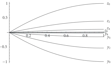
Example 3.2. Let us consider a problem

x(t)=sinx(t)+x(0.9t) + 1

32, t∈J=[0, 1],

x(0)=0, x(1)= −x(0.5).

0.2 0.4 0.6 0.8 1

1 0.5 0.5

1 z0

z2

z4

z8

y8

y4

y2

y0

Figure 3.1. Some iterations forExample 3.2.

Puty0(t)=t(t−2),z0(t)= −t(t−2). Then

y0(0)=z0(0)=0, y0(1)= −1<−3

4 = −z0(0.5), z0(1)=1> 3

4= −y0(0.5),

sin−t(t−2)−0.9t(0.9t−2) + 1

32≤sin(1) + 1 + 1

32<2=y 0(t),

sint(t−2)+ 0.9t(0.9t−2) + 1

32≥sin(−1)−1 + 1

32>−2=z0(t).

(3.14)

We show thaty0,z0are coupled lower and upper solutions of (3.13). Indeed, condition (3.1) holds. In view ofTheorem 3.1, problem (3.13) has, in segment [y0,z0], the minimal and maximal coupled quasisolutions.

InFigure 3.1, we see numerical results of some iterations algorithm fromTheorem 3.1. Numerical solutions have been found byMathematica 4.0. Solutions are interpolated by Lagrange interpolating polynomials to obtain values for deviating arguments. In this picture we have only iterationsyi,zifori=0, 2, 4, 8.

4. Generalization

Let us consider a boundary value problem

x(t)=gt,x(t),xα1(t),. . .,xαp(t)

≡Fx(t), t∈J=[0,T],

x(0)=0, x(T)=rx(γ) forγ∈(0,T),

(4.1)

whereg∈C(J×Rp+1_{,R),r,γare fixed numbers and functionsα}

i∈C(J,J) fori=1,. . .,p.

and maximal coupled quasisolutions of problem (4.1) are analogy of Definitions2.3,2.4, and2.5. Now we write analogue ofTheorem 3.1for the problem (4.1). We omit the proof of this theorem because it is similar to the one ofTheorem 3.1.

Theorem4.1. Letr≤0,g∈C(J×Rp+1_{,R), andα}

i∈C(J,J)fori=1,. . .,p. Lety0,z0be coupled lower and upper solutions of (4.1) andy0(t)≤z0(t),t∈J. Moreover, assume that

gt,u1,v1,. . .,vp

−gt,u1,v1,. . .,vp

≤0 (4.2)

fory0(t)≤u1≤u1≤z0(t),y0(αi(t))≤vi≤vi≤v0(αi(t))fori=1,. . .,p.

Then problem (4.1) has, in segment[y0,z0], the minimal and maximal coupled quasiso-lutions.

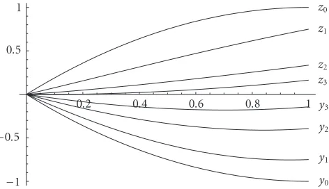
Example 4.2. ForJ=[0, 1], let us consider a problem

x(t)=0.4 sinx(t)+ 0.2x(0.9t) + 0.5 expx(√t)+ 1

32, t∈J,

x(0)=0, x(1)= −x(0.5).

(4.3)

Note thatα1(t)=0.9t,α2(t)=√t.Put y0(t)=t(t−2),z0(t)= −t(t−2). Theny0(0)=

z0(0)=0,y0(1)<−z0(0.5),z0(1)>−y0(0.5), and

0.4 sin−t(t−2)−0.20.9t(0.9t−2)+ 0.5 exp−√t(√t−2)+ 1 32

≤0.4 sin(1) + 0.2 + 0.5 exp(1) + 1

32≈1.93<2=y 0(t),

0.4 sint(t−2)+ 0.18t(0.9t−2) + 0.5 exp√t(√t−2)+ 1 32

≥0.4 sin(−1)−0.2 + 0.5 exp(−1) + 1

32≈−0.32>−2=z 0(t).

(4.4)

We see thaty0,z0are coupled lower and upper solutions of (4.3). Indeed,gsatisfies con-dition (4.2). In view ofTheorem 4.1, problem (4.3) has in segment [y0,z0] the minimal and maximal coupled quasisolutions. OnFigure 4.1we see results of first three iterations.

5. Result forr >0

We would like to transfer proof techniques used before to problem (1.1) withr >0. To get a similar result we have to change definitions.

Definition 5.1. A pair of functions y0,z0∈C2(J,R) are calledcoupledlower and upper solutions of (1.1) if

y0(t)≥Fz0(t), y0(0)≤0, y0(T)≤r y0(γ),

z0(t)≤F y0(t), z0(0)≥0, z0(T)≥rz0(γ),

(5.1)

0.2 0.4 0.6 0.8 1

1 0.5 0.5

1 z0

z1

z2

z3

y3

y2

y1

y0

Figure 4.1. Result of three iterations inExample 4.2.

Definition 5.2. A pair of functionsY,Z∈C2_{(J,R) are calledcoupled quasisolutions of} (1.1) if

Y(t)=FZ(t), Y(0)=0, Y(T)=rY(γ),

Z(t)=FY(t), Z(0)=0, Z(T)=rZ(γ),

(5.2)

wheret∈J.

We can proveTheorem 5.3by the same way as we provedTheorem 3.1.

Theorem5.3. Let f ∈C(J×R×R,R),r >0, andα∈C(J,J). Lety0,z0be coupled lower and upper solutions of (1.1) andy0(t)≤z0(t),t∈J. Moreover, assume that

ft,u1,v1

−ft,u1,v1

≤0 (5.3)

fory0(t)≤u1≤u1≤z0(t),y0(α(t))≤v1≤v1≤v0(α(t)).

Then problem (1.1) has, in segment[y0,z0], the minimal and maximal coupled quasiso-lutions.

6. Combination of coupled quasisolutions

It is turned out that we can combine some results of [4] with this work. In [4], it is assumed that f satisfies one-side Lipschitz condition with corresponding functional co-efficients.

assume that

M,N∈CJ, [0,∞), M(t)>0,t∈(0,T), (6.1)

ρ≡max

T

0

T

s

M(t) +N(t)dt

ds,

T

0

s

0[M(t) +N(t)]dt

ds

≤1, (6.2)

ft,e1,r1

−ft,e1,r1

≥ −M(t)e1−e1

−N(t)r1−r1

, (6.3)

wherey0(t)≤e1≤e1≤z0(t),y0(α(t))≤r1≤r1≤z0(α(t)).

Then problem (1.1) has, in segment[y0,z0], the minimal and maximal coupled quasiso-lutions.

Let us introduce the following operator:

F(x,y)(t)=ft,x(t),xα(t),y(t),yβ(t), (6.4)

whereα,β∈C(J,J).

Now we consider a problem

x(t)=F(x,x)(t), t∈J=[0,T],

x(0)=0, x(T)=rx(γ) withγ∈(0,T), r≤0,

(6.5)

where f ∈C(J×R4_{,R),r,γare fixed numbers andα,β∈C(J,J).}

We will combine definitions of coupled lower and upper solutions with coupled lower and upper solutions.

Definition 6.2. A pair of functions y0,z0∈C2(J,R) is calledcoupled lower and upper solutions of (6.5) if

y0(t)≥F(z0,y0)(t), y0(0)≤0, y0(T)≤rz0(γ),

z0(t)≤F(y0,z0)(t), z0(0)≥0, z0(T)≥r y0(γ),

(6.6)

wheret∈J.

Definition 6.3. A pair of functionsY,Z∈C2_{(J,R) is calledcoupled quasisolutionsof (6.5)} if

Y(t)=F(Z,Y)(t), Y(0)=0, Y(T)=rZ(γ),

Z(t)=F(Y,Z)(t), Z(0)=0, Z(T)=rY(γ),

(6.7)

wheret∈Jand 0< γ < T.

Theorem6.4. Let f ∈C(J×R4_{,R),r≤0, andα,β∈C(J,J). Lety}

0,z0be coupled lower and upper solutions of (6.5) andy0(t)≤z0(t),t∈J. Moreover, assume that

ft,u1,v1,u2,u3

−ft,u1,v1,u2,u3

wherey0(t)≤u1≤u1≤z0(t),y0(α(t))≤v1≤v1≤z0(α(t)), and

ft,w1,w2,e1,r1−ft,w1,w2,e1,r1≥ −M(t)e1−e1−N(t)r1−r1, (6.9)

wherey0(t)≤e1≤e1≤z0(t),y0(β(t))≤r1≤r1≤z0(β(t))and forM,Nconditions (6.1) and (6.2) hold.

Then problem (6.5) has, in segment[y0,z0], the minimal and maximal coupled quasiso-lutions.

To prove this theorem we apply the way of this paper combined with [4] and therefore we omit the proof. Note thatynandznare defined by

y_n(t)=Fzn−1,yn−1(t) +M(t)yn(t)−yn−1(t)+N(t)ynβ(t)−yn−1β(t), t∈J,

yn(0)=0, yn(T)=rzn−1(γ),

z_n(t)=Fyn−1,zn−1(t) +M(t)zn(t)−zn−1(t)+N(t)znβ(t)−zn−1β(t), t∈J,

zn(0)=0, zn(T)=r yn−1(γ).

(6.10)

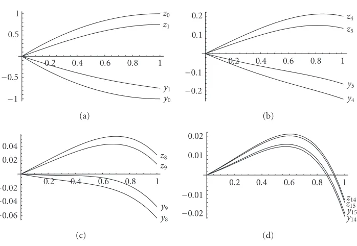
Example 6.5. Let us consider a problem which is combination of examples from this paper and from [4], so we omit checking the assumptions about f,

x(t)=sinx(t)+x(0.9t) + 1

32+x(t) sin(t) + 0.4x(0.5t) cos(t)−tsin(t), t∈J=[0, 1]

x(0)=0, x(1)= −x(0.5).

(6.11)

Put y0(t)=t(t−2), z0(t)= −t(t−2). It is easy (just like before) to show that y0, z0 are coupled lower and upper solutions of (6.11). Thus problem (6.11) has, in segment [y0,z0], the minimal and maximal coupled quasisolutions. OnFigure 6.1we see some chosen pairs of numerical approximations of quasisolutions of problem (6.11).

Remark 6.6. There is no problem to investigate problem (6.5) whenr >0.

7. From minimal and maximal quasisolutions to solution

0.2 0.4 0.6 0.8 1

1 0.5 0.5

1 z0

z1

y1

y0

(a)

0.2 0.4 0.6 0.8 1

0.2 0.1 0.1

0.2 z4

z5

y5

y4

(b)

0.2 0.4 0.6 0.8 1

0.06 0.04 0.02 0.02 0.04

z8

z9

y9

y8

(c)

0.2 0.4 0.6 0.8 1

0.02 0.01 0.01 0.02

z14

z15

y15

y14

(d)

Figure 6.1. Chosen pairs of quasisolutions of problem (6.11).

Lemma7.1. Assume thatγ∈(0,T)and0≤kγ < T.Let p∈C2_{(J,R),B∈C(C}2_(J,R)× J,R), and

p(t)≥B(p,t), t∈J,

p(0)≤0, p(T)≤k p(γ).

(7.1)

Then functionpsatisfies the following inequality:

p(t)≤ kt

T−kγ

γ

0

s

0B(p,τ)dτ ds+

t

0

s

0B(p,τ)dτ ds− t T−kγ

T

0

s

0B(p,τ)dτ ds. (7.2)

Proof. We replace problem (7.1) by

p(t)=B(p,t) +A, t∈J,

p(0)=a, p(T)=k p(γ) +b

(7.3)

withA≥0,a≤0,b≤0.Integrating it two times on [0,t], we obtain

p(t)=a+p(0)t+1 2At

2₊ t 0

s

To calculatep(0), we have to use boundary conditions. Thus

p(t)=1 2At

_γ2_k−T2

T−kγ +t

+ kt T−kγ

γ

0

s

0B(p,τ)dτ ds

+

t

0

s

0B(p,τ)dτ ds− t T−kγ

T

0

s

0B(p,τ)dτ ds

+a

1 +t(k−1) T−kγ

+ bt

T−kγ.

(7.5)

Note that ifk≥1, then 1 +t(k−1)/(T−kγ)≥1.Now if 0≤k <1, then

1 +t(k−1) T−kγ ≥1 +

T(k−1) T−kγ =

k(T−γ)

T−kγ ≥0. (7.6)

In view of the inequalityγ2_{k≤γTk, assumptionsa≤0,b≤0, and (7.5), we obtain}

p(t)≤1

2At(t−T) + kt T−kγ

γ

0

s

0B(p,τ)dτ ds

+

t

0

s

0B(p,τ)dτ ds− t T−kγ

T

0

s

0B(p,τ)dτ ds.

(7.7)

Hence we have (7.2) sinceA≥0.It ends the proof.

To use this lemma we will additionally assume that f satisfies one-side Lipschitz con-dition with corresponding functional coefficients.

Theorem7.2. Assume that all assumptions ofTheorem 6.4hold. LetT >−rγ.In addition, assume that there exist functionsL1,L2,L3,L4∈C(J,R+)such that

T T−kγ

T

0

s

0

L1(t) +L2(t) +L3(t) +L4(t)dt

ds <1, (7.8)

−L1(t)u1−u1

−L2(t)v1−v1

≤ft,u1,v1,u2,u3

−ft,u1,v1,u2,u3

, (7.9)

wherey0(t)≤u1≤u1≤z0(t),y0(α(t))≤v1≤v1≤z0(α(t)), and L3(t)e1−e1

+L4(t)r1−r1

≥ft,w1,w2,e1,r1

−ft,w1,w2,e1,r1

, (7.10)

wherey0(t)≤e1≤e1≤z0(t),y0(β(t))≤r1≤r1≤z0(β(t)). Then problem (6.5) has, in segment[y0,z0], exactly one solution.

Proof. FromTheorem 6.4, we know that problem (6.5) has, in segment [y0,z0], the min-imal and maxmin-imal coupled quasisolutionsyandzandy(t)≤z(t) onJ.Letp(t)=z(t)−

and (7.10), we get

p(t)=F(y,z)(t)−F(z,z)(t) +F(z,z)(t)−F(z,y)(t)

≥ −L1(t)p(t)−L2(t)pα(t)−L3(t)p(t)−L4(t)pβ(t)≡B(p,t).

(7.11)

It is obvious thatB(p,t)≤0 fort∈J. FromLemma 7.1, we obtain

p(t)≤ kt T−kγ

γ

0

s

0B(p,τ)dτ ds+

t

0

s

0B(p,τ)dτ ds− t T−kγ

T

0

s

0B(p,τ)dτ ds (7.12)

withk= −r.

Note that the first two elements of (7.12) are negative, so we omit them. Hence

p(t)≤ − t

T−kγ

T

0

s

0B(p,τ)dτ ds, t∈J. (7.13) Suppose, that maxt∈Jp(t)=p(t1)=D >0. From (7.13), we obtain

D≤ t1 T−kγ

T

0

s

0

L1(t) +L3(t)pt1

+L2(t)pαt1

+L4(t)pβt1

dt ds

≤ TD

T−kγ

T

0

s

0

L1(t) +L2(t) +L3(t) +L4(t)dt ds,

(7.14)

so

D

1−_T−T_kγ T

0

s

0

L1(t) +L2(t) +L3(t) +L4(t)dt

ds

≤0. (7.15)

By condition (7.8), we getD≤0.It is a contradiction.

It proves thatp(t)=0 fort∈J. Thusy≡zandyis a solution of problem (6.5).

Remark 7.3. For example, ifLi(t)=Li,i=1, 2, 3, 4, then condition (7.8) takes the form

L1+L2+L3+L4<2 T+rγ

T3 . (7.16)

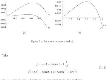
Example 7.4. Let us consider a problem like inExample 6.5with a little modification of the boundary condition, namely,

x(t)=sinx(t)+x(0.9t) + 1

32+x(t) sin(t) + 0.4x(0.5t) cos(t)−tsin(t), t∈J=[0, 1]

x(0)=0, x(1)= −x(0.3).

(7.17)

0.2 0.4 0.6 0.8 1

0.03 0.02 0.01 0.01 0.02 0.03

z6

y6

(a)

0.2 0.4 0.6 0.8 1

0.01 0.005 0.005 0.01 0.015 0.02

z16

y16

(b)

Figure 7.1. Iterations number 6 and 16.

Take

f1(t,u,v)=sin(u) +v+ 1 32,

f2(t,e,r)=esin(t) + 0.4rcos(t)−tsin(t).

(7.18)

Letu1≤u1andv1≤v1. Then from a mean value theorem, we obtain

f1

t,u1,v1

−f1

t,u1,v1

=sinu1

−sin(u) +v1−v1≥ −1

u−u1

−1v−v1

,

(7.19)

thusL1(t)=1,L2(t)=1. Lete1≤e1andr1≤r1. Then

f2

t,e1,r1

−f1

t,e1,r1

=e1sin(t)−e1sin(t) + 0.4r1cos(t)−0.4r1cos(t)

= −sin(t)e1−e1

−0.4 cos(t)r1−r1

,

(7.20)

thusL3(t)= −sin(t),L4(t)= −0.4 cos(t). Thus conditions (7.9) and (7.10) are satisfied. It is easy to show that

1 1−0.3

1

0

s

0

2−sin(t)−0.4 cos(t)dt

ds <1. (7.21)

OnFigure 7.1, we present approximations of solutions (iterations 6 and 16). Maximal differences between them are

max

t∈J

_{y6(t)−z6(t)≈0.035, max}

t∈J

References

[1] W. Ding, M. Han, and J. Mi, Periodic boundary value problem for the second-order impulsive functional differential equations, Computers & Mathematics with Applications50(2005), no. 3-4, 491–507.

[2] T. Jankowski, Advanced differential equations with nonlinear boundary conditions, Journal of Mathematical Analysis and Applications304(2005), no. 2, 490–503.

[3] ,On delay differential equations with nonlinear boundary conditions, Boundary Value Problems2005(2005), no. 2, 201–214.

[4] ,Solvability of three point boundary value problems for second order differential equations with deviating arguments, Journal of Mathematical Analysis and Applications312(2005), no. 2, 620–636.

[5] ,Boundary value problems for first order differential equations of mixed type, Nonlinear Analysis64(2006), no. 9, 1984–1997.

[6] D. Jiang, M. Fan, and A. Wan,A monotone method for constructing extremal solutions to second-order periodic boundary value problems, Journal of Computational and Applied Mathematics136 (2001), no. 1-2, 189–197.

[7] D. Jiang and J. Wei,Monotone method for first- and second-order periodic boundary value problems and periodic solutions of functional differential equations, Nonlinear Analysis50(2002), no. 7, 885–898.

[8] D. Jiang, P. Weng, and X. Li,Periodic boundary value problems for second order differential equa-tions with delay and monotone iterative methods, Dynamics of Continuous, Discrete & Impulsive Systems. Series A10(2003), no. 4, 515–523.

[9] V. Kolmanovskii and A. Myshkis,Introduction to the Theory and Applications of Functional Dif-ferential Equations, Mathematics and Its Applications, vol. 463, Kluwer Academic, Dordrecht, 1999.

[10] G. S. Ladde, V. Lakshmikantham, and A. S. Vatsala,Monotone Iterative Techniques for Nonlinear Differential Equations, Monographs, Advanced Texts and Surveys in Pure and Applied Mathe-matics, vol. 27, Pitman, Massachusetts, 1985.

[11] J. J. Nieto and R. Rodr´ıguez-L ´opez,Existence and approximation of solutions for nonlinear func-tional differential equations with periodic boundary value conditions, Computers & Mathematics with Applications40(2000), no. 4-5, 433–442.

[12] ,Remarks on periodic boundary value problems for functional differential equations, Jour-nal of ComputatioJour-nal and Applied Mathematics158(2003), no. 2, 339–353.

T. Jankowski: Department of Differential Equations, Gdansk University of Technology, 11/12 G. Narutowicz Street, 80-952 Gda ´nsk, Poland

E-mail address:[email protected]

W. Szatanik: Department of Differential Equations, Gdansk University of Technology, 11/12 G. Narutowicz Street, 80-952 Gda ´nsk, Poland