Fast comparison of IS radar code sequences for lag proﬁle inversion

(1)

www.ann-geophys.net/26/2291/2008/ © European Geosciences Union 2008

Annales

Geophysicae

Fast comparison of IS radar code sequences for lag profile inversion

M. S. Lehtinen1, I. I. Virtanen2, and J. Vierinen1

1_{Sodankyl¨a Geophysical Observatory, 99600, Sodankyl¨a, Finland}

2_{Department of Physical Sciences, University of Oulu, P.O. Box 3000, 90014, Finland}

Received: 3 January 2008 – Revised: 27 May 2008 – Accepted: 4 June 2008 – Published: 5 August 2008

Abstract. A fast method for theoretically comparing the

pos-teriori variances produced by different phase code sequences in incoherent scatter radar (ISR) experiments is introduced. Alternating codes of types 1 and 2 are known to be optimal for selected range resolutions, but the code sets are inconve-niently long for many purposes like ground clutter estimation and in cases where coherent echoes from lower ionospheric layers are to be analyzed in addition to standard F-layer spec-tra.

The method is used in practice for searching binary code quads that have estimation accuracy almost equal to that of much longer alternating code sets. Though the code se-quences can consist of as few as four different transmission envelopes, the lag profile estimation variances are near to the theoretical minimum. Thus the short code sequence is equally good as a full cycle of alternating codes with the same pulse length and bit length. The short code groups can-not be directly decoded, but the decoding is done in connec-tion with more computaconnec-tionally expensive lag profile inver-sion in data analysis.

The actual code searches as well as the analysis and real data results from the found short code searches are explained in other papers sent to the same issue of this journal. We also discuss interesting subtle differences found between the different alternating codes by this method. We assume that thermal noise dominates the incoherent scatter signal.

Keywords. Radio science (Ionospheric physics; Signal

pro-cessing; Instruments and techniques)

1 Introduction

In incoherent scatter radar measurements the desired range resolution is often much better than the available pulse length Correspondence to: M. S. Lehtinen

([email protected])

of the radar. In order to maximize the statistics of the results special coding methods like alternating codes have been de-veloped to allow the radar to be used at full duty cycle and still produce range resolutions much shorter than the pulse length used (Lehtinen and H¨aggstrom, 1987). Typical fea-tures of these kinds of methods are:

– Long pulses are modulated by a binary phase pattern,

which gives range resolution approximately equal to the baud length of this pattern.

– This requires relatively little computation because

the resolution is achieved by a simple summa-tion/subtraction procedure of the corresponding lag products of all the codes in the code set.

Then there are the newer codes that have the advantage that the code set can contain fewer codes, especially important when the equivalent alternating code set has many codes (Virtanen et al., 2007; Damtie et al., 2002). These codes:

1. preserve the range resolution that the equivalent alter-nating code set provides,

2. but do not allow this resolution to be accessed by such a simple procedure as adding/subtracting corresponding lag products.

3. Instead they require a possibly computationally inten-sive inversion, and thus are practical now, but were not two decades ago.

4. Since these codes are found by a search technique, com-putationally intensive due to the vast number of possible code sets, it is necessary to make this process efficient. 5. The important thing is not whether data from a code

(2)

6. Since different code sets degrade the SNR by vastly dif-ferent amounts, a very important part of the search tech-nique is the evaluation of the degradation.

7. This paper describes a fast method for doing this, a method that is not necessarily as accurate as slower methods, but nonetheless is good enough to allow good code sets to be separated from the vast number of bad code sets.

We also use the developed comparison method to discuss some interesting differences found between strong alternat-ing codes, weak alternatalternat-ing codes (Lehtinen and H¨aggstrom, 1987) and alternating codes of type 2 (Sulzer, 1993), seen in the way they perform in terms of variance behavior when post-integrating lag profile data to coarser resolutions.

The actual (accurate) method for decoding the codes is to apply linear statistical inversion to the lag profiles measure-ments, which represent the desired unknown plasma scatter-ing lag profiles convolved with the range ambiguity functions corresponding to the different lagged products of the codes in the code group under study. If the lag profiles are very long, the faster method of inversion can be based on Fourier trans-forms of the profiles. These methods will fail near the ends of the profiles, but they provide us with a much faster way to estimate the variance behaviour of the inversion process with results valid if we do not worry about what happens near the ends of the profiles. Because the code groups are searched with time-consuming computer searches the speed obtained this way is essential.

The linear statistical inversion based method is described in Virtanen et al. (2007). These methods are developed to-wards general-purpose experiments in another paper in this special issue (Virtanen et al., 2008). There are also other re-lated papers in this special issue:

Another paper (Vierinen et al., 2008) describes the effi-cient search algorithms used for actual searches of the code quads. We also discuss the advantages of using polyphase codes and amplitude modulation instead of binary modula-tion.

We discuss the possibility of doing inversion analysis of echo amplitude data to solve for the scattering amplitudes in-stead of correlation properties of the target (Vierinen et al., 2008b). This way of analysis is advantageous with very nar-row targets like meteor heads and narnar-row ionospheric layers. We have shown that the new experiments can be used to-gether with advanced MCMC (Markov Chain Monte Carlo) techniques combined with ionospheric models to do analy-sis in cases beyond the capabilities of traditional GUISDAP analysis or the lag profile inversion (Kero et al., 2008).

We have also generalized binary alternating codes to a general number of phases (Markkanen et al., 2008). This paper is purely a generalization of the classical way of cod-ing and decodcod-ing by summation – with no need for inversion methods.

2 Code selection

The focus of the code selection is to find the code sequences that produce minimum posteriori variances for the inverted lag profiles. Starting from the scattering process happening in the ionosphere it is possible to derive an analytical for-mula for the posteriori variance of any lag value for any code sequence. For each code length and each lag value the vari-ance has a theoretical minimum. By comparing the calcu-lated variances of different codes to the minimum variances at all lag values the best codes can be selected.

We use here a discrete formalism, where all times (and ranges which are also specified as corresponding times) are represented as integers. The discrete formalism can be derived from the continuous-time formalism developed in (Lehtinen, 1986; Lehtinen and Huuskonen, 1996) by study-ing samples of signals given byzi=_1t1 R_i1t(i+1)1tz(t )dtin the

limit1t→0.

2.1 Scattering from the ionosphere

The scattering coefficient of an ionospheric plasma element is noted withxr,t, whereris signal travel time to the

scatter-ing volume and back andtis time. The scattering is modeled as a zero mean stochastic process with covariance

hxr;txr0_;_t0i =δ_rr0σt−t

0

r , (1)

whereδrr0 is the Kronecker delta andxis the complex

con-jugate ofx. Plasma scattering properties are modeled by the plasma autocorrelation functionσ_rt−t0.

In a practical incoherent scatter experiment the illumina-tion by radio waves is not continuous, but the radar sends phase coded pulses to the ionosphere. The scattered signal is recorded in the form of discrete IQ-samples (raw data).

If the discretization step1t is small enough, the ampli-tude ambiguity function for range simplifies to be equal to the transmission waveform envt and thus the received

com-plex signal is a weighted sum of the scattering coefficients

zq=

∞

X

r=−∞

envrxq−r;q+εq, (2)

where envq is the complex transmission envelope and εq

the measurement error due to thermal noise. It’s correlation properties are expressed by

hεqεq0i =

C

1tδqq0, (3)

whereCis a constant depending on the amplitude of the ther-mal noise.

2.2 Lag profiles and inversion

In an incoherent scatter radar experiment lagged products of the received signal and its complex conjugate,

(3)

are calculated. Using Eq. (1) the expectations of the lagged products can be written in the form

h mq;τi = hzqzq−τi

= h

∞

X

r=−∞

(envrxq−r;q+εq)·

∞

X

s=−∞

(envsxq−τ−s;q−τ+εq−τ)i

=

∞

X

r=−∞

envrenvr−τσqτ−r

=

∞

X

r=−∞

Wr;τσqτ−r. (5)

The expectations of the terms containing measurement errors are zeros.

A range profile of plasma autocorrelation functionσ_qτ with a fixed value of time lagτ is called a “lag profile”. In the analysis several lag profilesσ_qτ with selected values ofτ are solved as separate problems to sample the whole plasma au-tocorrelation function. The difference between a measured ambiguous lagged product and its expectation is

mq;τ = hmq;τi +εq;τ

=

∞

X

r=−∞

Wr;τσqτ−r+εq;τ. (6)

The error term in Eq. (6) is rather complicated. The fourth moment’s theorem for complex Gaussian processes imply

hεq;τεq0_;_τ0i = hz_qz_q0₋_τ0ihz_q0z_q₋_τi

hεq;τεq0_;_τ0i = hz_qz_q0ihz_q₋_τz_q0₋_τ0i. (7)

These formulas, represented in terms of the real and imagi-nary parts of the lag profile expectationshmq;τican be found

in the references cited above. The mutual correlations of the error term εq;τ between both different lags and

differ-ent ranges can be fully explained by these formulas. This is the correct way to model the self-noise of the lag profile estimates, when the signal-to-noise ratio is not very low.

For the purposes of this study, we assume a very low signal-to-noise ratio, and the error term simplifies to

hRe(εq;τ)Re(εq0_;_τ0)i =

C2

1t2δqq0(δτ τ0+δτ0)

hIm(εq;τ)Im(εq0_;_τ0)i =

C2

1t2δqq0δτ τ0(1−δτ0)

hRe(εq;τ)Im(εq0_;_τ0)i =0, (8)

ifτ≥0 andτ0≥0. The lag profile estimates are thus indepen-dent of each other if either the lag values or the range values differ. The variance of the zero lag profile is two times the variance of the other lag profiles. Negative values of the lags are completely dependent on the positive values, being com-plex conjugates of each other.

The Fourier transform of the measured lag profile is

˜

mτ(ω)=

∞

X

q=−∞

eiqω

∞

X

r=−∞

Wr;τσqτ−r+εq;τ !

= ˜στ(ω)W˜τ(ω)+ ˜ετ(ω) (9)

as indicated by the convolution theorem of the Fourier trans-forms. The Fourier transform of the plasma autocorrelation functionσ_rτ is not the plasma scattering spectrum, because the transform is taken with respect to the range variable r, not the time lagτ.

The inversion solution (and the error term) of the Fourier transform of the unknown lag profile is

˜

στ(ω)= m˜τ(ω)

˜

Wτ(ω)

− ε˜τ(ω)

˜

Wτ(ω)

. (10)

2.3 Posteriori noise

Now lets take a closer look at the transform of the noise, i.e. the last term in Eq. (9). Using Eq. (8) its covariance can be written as

h˜ετ(ω)ε˜τ(ω0)i =

∞

X

q=−∞

eiq(ω−ω0)

=2π δ(ω−ω0). (11)

The latter term in Eq. (10) is the Fourier transform of the posteriori noise. By taking the inverse transform we get the posteriori noise in time domain

ξ =F−1(ε˜τ(ω)/W˜τ(ω)). (12)

The covariance of the posteriori noise in Eq. (12) is

hξpξqi =

1

(2π )2 2π Z

0 2π Z

0

e−ipωeiqω0hε˜τ(ω) ˜

Wτ(ω)

˜ ετ(ω0)

˜ Wτ(ω0)

idωdω0

= 1

2π 2π Z

0

e−i((p−q)ω) 1

| ˜Wτ(ω)|2

dω. (13)

The previous holds for a single transmission envelope that leads to a single range ambiguity function for each lag value. In case of several envelopes, i.e. a code sequence longer than one, each of the envelopes produces a different range am-biguity function for each lag value. From a sequence ofN

codes, equations

W_ru_;_τ =envu_renvu_r₋_τ, (14)

u = 1. . . N, are produced. Each of these range ambiguity

functions produce an equation similar to Eq. (6)

mu_q_;_τ =

∞

X

r=−∞

(4)

5 10 15 20

0.00

0.02

0.04

0.06

0.08

0.10

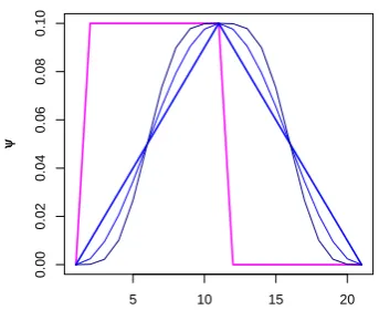
[image:4.595.81.253.60.200.2]

ψψ

Fig. 1. Range integration averaging kernels used in the

calcula-tions. The boxcar kernel (magenta) was not used in the subsequent calculations. The triangle kernel (thick blue) seemed to perform best while the shaped kernel (thin blue) and the iterated sin-shaped kernel (dark blue) performed slightly worse. The results corresponding to the last three kernels are shown with correspond-ingly colored curves in the results.

and has a Fourier transform

˜

mu_τ(ω)= ˜στ(ω)W˜_τu(ω)+ ˜εu_τ(ω). (16)

The inversion solution (and the error term) for the Fourier transform of the lag profile using all the measurements can now be written as

˜

στ(ω)=

PN

u=1W˜τu(ω)m˜uτ(ω) PN

u=1| ˜Wτu(ω)|2

+ ε˜τ(ω)

q PN

u=1| ˜Wτu(ω)|2

, (17)

whereε˜τ(ω)is the Fourier transform of a normalized white

noise. The posteriori noise covariance is

hξpξqi =

1 2π

2π Z

0

e−i(p−q)ω

PN

u=1| ˜Wτu(ω)|2

dω. (18)

From Eq. (18) we get the posteriori variance of the inversion result

hξpξpi =

1 2π

2π Z

0

1

PN

u=1| ˜Wτu(ω)|2

dω. (19)

that has a minimum

hξpξpi ≥

N X

u=1

∞

X

r=−∞

|W_ru_;_τ|2

!−1

. (20)

2.4 Proof of the accuracy limit

It is surprisingly easy to see that the inequality (20) must be true. For this, let us assume that the only unknown lag profile value isσ_qτ and that we know all the other values ofσ_pτ, if

p6=q. Our only unknown then appears in the measurement Eq. (15) multiplied by all the valuesW_ru_;_τ with 1≤u≤N and

−∞<r<∞.

As the error terms in Eq. (20) are assumed normalized and independent, the inversion accuracy for this only unknown variable is easily seen to be equal to the right hand side of Eq. (20).

If we now drop the assumption about exact knowledge of the other scattering termsσ_pτ,p6=q, the estimation accuracy of the previously only unknown cannot get any better. Thus, the inequality in Eq. (20) must be true.

The inequality (20) is also a consequence of the well-known mathematical fact that the harmonic mean of numbers is smaller or equal to the arithmetic mean of the numbers. 2.5 Code selection criteria

Now we have finally arrived to the formulas that can be used in comparing different code sequences. The efficiency of a code is defined as ratio of the minimum posteriori variance as defined in Eq. (20) and the actual posteriori variance of the code under study,

R=

PN

u=1

P∞

r=−∞|Wru;τ|

2−1

1 2π

2π R

0 1

PN

u=1| ˜Wτu(ω)|2

dω

. (21)

In practical calculations the Fourier transform of the range ambiguity function can be handled with DFT. When the in-tegral in the denominator is written in discrete form using Riemann sum, we get the form

PN

u=1

P∞

r=−∞|Wru;τ|2 −1

1

M PM−1

q=0 1

PN u=1| ˜Wτu;q|2

→RasM→ ∞. (22)

In the case of binary code groups the nominator can be sim-plified even further. The amplitude of range ambiguity func-tion is|W_ru_;_τ|=1 in all non-zero parts of the function. If the codes haveNbbits and only the full lags (multiples of the bit

length) are studied, Eq. (22) can be written in form

(N (Nb−τ ))−1

1

M PM−1

q=0 PN 1 u=1| ˜Wτu;q|2

→RasM→ ∞. (23)

2.6 Range integration

(5)

ψare used to get the range integrated values. The convolu-tion gives an extra term to the posteriori variance (Eq. 19), so that the variance of the integrated lag profile is

hξpξpi =

1 2π

2π Z

0

| ˜9(ω)|2

PN

u=1| ˜Wτu(ω)|2

dω, (24)

where9(ω)˜ is the Fourier transform of the averaging con-volution kernel9. The discrete version of this formula is easily obtained by replacing 1/2π by 1/Mand the integral overωby summation over the discrete FFT valuesωi. A very

natural choise for the averaging kernel would be the boxcar function

9box(n)= 1

Nr

, if 0≤n<Nr, 9(n)=0 otherwise. (25)

However, it was discovered that the boxcar shape performed very badly. For this reason we defined a triangular averaging function by setting

1Nr(n)=n/Nr, if 1≤n≤Nr

1Nr(n)=1−n/Nr, if Nr<n≤2Nr

1Nr(n)=0, otherwise (26)

and

91(n)=1Nr/Nr. (27)

Moreover, a sinusoidal shaped averaging function as well as an iterated sinusoidal averaging function (rather close to box-car) were defined by

9sin(n)=sinπ

21Nr(n) 2

(28) and

9sin sin(n)=sin

_π

2 sin

π

21Nr(n)

22

. (29)

All these kernels are shown in Fig. 1.

3 Numerical results

As our goal was to find a code sequence of 15 bauds of 10µs duration, we first evaluated such a code set of randomly cho-sen binary bauds. The results for the randomly chocho-sen code set are shown in Fig. 3. We have plotted the variances of the experiments as a function of range integration. The results from the simple and fast formula (22) or (23) are shown by the red curve and the results for more careful calculations, modelling the signal values as 5 samples taken for each baud by the blue curves. The three different rows of the curves cor-respond to a different number of fractional lag profiles taken to represent each full lag value.

The formulas used for both cases are the same. The main difference is that in the simple case we use 1 discrete sample

to represent each baud, while in the more realistical case we use 5 samples to represent each baud. Moreover, in the more realistic case the full lags are multiples of 5 samples and each of them is estimated using fractional lags around this exact multiple of 5 samples.

It can be seen that realistic curves rather well follow the fast formula (22) or (23), but that there are occasionally even significant discrepancies between them. However, we feel this anyway justifies the use of rapid formulae in extensive computer searches.

4 Careful explanation of the result figures

The main contribution of this paper, in addition to Eqs. (22) or (23) and (24) are the numerical results shown in form of matrices of curves for different situations. As these graph-ics contain a great wealth of information, it is necessary to carfully explain everything shown in them.

The figures consist of three of five rows of panes. The first row shows the pulse forms and the range ambiguity func-tions. The second row shows the squared moduli of the Fourier transforms of the individual range ambiguities, nor-malized by dividing by the number of codes and the sum of these individual Fourier transforms. This sum can be consid-ered as the average Fisher information of the inverse convo-lution problem. The last 1 or 3 rows show how the results be-have when range-integrated to various resolutions. We show the behaviour for both the simplest formula as the red curve as well as a set of other curves – calculated more carefully by discretizing the analysis to 5 steps for each baud in the code. We always show the results for calculation of fractional lags

±2,±1 and 0 and in the 5-row panels also for other kinds of fractional lag sets involved in the analysis.

4.1 First line of figure panes

Here we simply show the range ambiguity functions for all full lags. LAG 0 is different, as the range ambiguity function is just a constant of the length of the pulse itself and it is not very informative to show it. Instead, we plot the codes themselves in that position. To emphasize the difference, we plot the code in blue. At the top of these panels we also print the relevant full lag number.

4.2 Second line of figure panes

(6)

Index

LAG 0

0.5

1.0

1.5

Index max= 4.00 min= 0.03 R= 0.420

1

2

Index

V=1/R= 2.382

V(1)= 2.041 V(20)= 0.196

1

2

Index

V=1/R= 2.382

V(1)= 1.849 V(20)= 0.214

5 15

1

2

V=1/R= 2.382

V(1)= 1.714 V(20)= 0.236

Index

NULL

LAG 1

Index

NULL

max= 1.00 min= 1.00 R= 1.000

Index

NULL

V=1/R= 1.000

V(1)= 1.121 V(20)= 0.567

Index

NULL

V=1/R= 1.000

V(1)= 1.221 V(20)= 0.505

5 15

NULL

V=1/R= 1.000

V(1)= 1.293 V(20)= 0.455

Index

NULL

LAG 2

Index

NULL

max= 1.00 min= 1.00 R= 1.000

Index

NULL

V=1/R= 1.000

V(1)= 1.155 V(20)= 0.674

Index

NULL

V=1/R= 1.000

V(1)= 1.307 V(20)= 0.677

5 15

NULL

V=1/R= 1.000

V(1)= 1.408 V(20)= 0.679

Index

NULL

LAG 3

Index

NULL

max= 1.00 min= 1.00 R= 1.000

Index

NULL

V=1/R= 1.000

V(1)= 1.061 V(20)= 0.669

Index

NULL

V=1/R= 1.000

V(1)= 1.112 V(20)= 0.669

5 15

NULL

V=1/R= 1.000

V(1)= 1.142 V(20)= 0.670

Index

NULL

LAG 4

Index

NULL

max= 1.00 min= 1.00 R= 1.000

Index

NULL

V=1/R= 1.000

V(1)= 1.053 V(20)= 0.668

Index

NULL

V=1/R= 1.000

V(1)= 1.100 V(20)= 0.668

5 15

NULL

V=1/R= 1.000

V(1)= 1.130 V(20)= 0.668

Index

NULL

LAG 5

Index

NULL

max= 1.00 min= 1.00 R= 1.000

Index

NULL

V=1/R= 1.000

V(1)= 1.053 V(20)= 0.668

Index

NULL

V=1/R= 1.000

V(1)= 1.100 V(20)= 0.668

5 15

NULL

V=1/R= 1.000

V(1)= 1.130 V(20)= 0.668

Index

NULL

LAG 6

Index

NULL

max= 1.00 min= 1.00 R= 1.000

Index

NULL

V=1/R= 1.000

V(1)= 1.031 V(20)= 0.715

Index

NULL

V=1/R= 1.000

V(1)= 1.055 V(20)= 0.758

5 15

NULL

V=1/R= 1.000

[image:6.595.98.501.60.425.2]

V(1)= 1.084 V(20)= 0.805

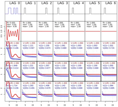
Fig. 2. Evaluation of a simple multiple-pulse type code.

If the ambiguity is a Kronecker delta of unit magnitude, the corresponding Fisher information is a constant one in Fourier side. Thus, a constant one represents a set of codes representing exactly the same kind of information that can be obtained from a single unit-strength pulse pair. A con-stant unit value here represents a perfect code set in the sense that the statistical properties of the analysis result are exactly equal to those corresponding to a simple pulse pair. However, we have normalized this curve by dividing it by the length of the ambiguity function – so it actually means that a constant unit value means pulse compression perfectly done with a apparent power corresponding to the length of the ambiguity function.

Please, note that the frequency axis is that of the FFT soft-ware: zero frequency corresponds to the left side of the figure while small negative frequencies are found on the right side of the x-axis. The center of the x-axis corresponds to the highest frequencies seen with the time discretization chosen.

The Fourier side information is easily interpreted in terms of what happens with range integration. If we have much in-formation at zero or low frequencies, it is obvious that range integration should perform well. This happens clearly in lag 8 in Fig. 4. Also, zero lags integrate well if fractional lags are taken into account. For the simple discrete case zero lags are singular and integration cannot help, except for the case of integration length equal to pulse length, which is seen as the downward spike on the red curve in some panels. On the other hand, having little information at DC results in very bad range integration results. This is remarkably clear for lags 5 and 10 in Fig. 3.

4.3 Last rows of figure panes

(7)

Index

LAG 0

0.5

1.0

1.5

Index max= 15.00 min= 0.00 R= 0.000 1 2 Index V=1/R= 3003.267 V(1)= 11.622 V(20)= 0.101 1 2 Index V=1/R= 3003.267 V(1)= 6.187 V(20)= 0.108 5 15 1 2 V=1/R= 3003.267 V(1)= 3.996 V(20)= 0.128 Index NULL

LAG 1

Index

NULL

max= 2.57 min= 0.35 R= 0.763 Index NULL V=1/R= 1.311 V(1)= 1.546 V(20)= 1.560 Index NULL V=1/R= 1.311 V(1)= 1.665 V(20)= 1.055 5 15 NULL V=1/R= 1.311 V(1)= 1.718 V(20)= 0.611 Index NULL

LAG 2

Index

NULL

LAG 3

Index

NULL

LAG 4

Index

NULL

LAG 5

Index

NULL

LAG 6

Index

NULL

LAG 7

Index

NULL

LAG 8

Index

NULL

LAG 9

Index

NULL

max= 1.68 min= 0.52 R= 0.848 Index NULL V=1/R= 1.180 V(1)= 1.335 V(20)= 1.296 Index NULL V=1/R= 1.180 V(1)= 1.465 V(20)= 1.469 5 15 NULL V=1/R= 1.180 V(1)= 1.530 V(20)= 1.459 Index NULL LAG 10 Index NULL

[image:7.595.46.552.62.280.2]

max= 1.00 min= 1.00 R= 1.000 Index NULL V=1/R= 1.000 V(1)= 1.108 V(20)= 0.834 Index NULL V=1/R= 1.000 V(1)= 1.195 V(20)= 0.957 5 15 NULL V=1/R= 1.000 V(1)= 1.270 V(20)= 1.052

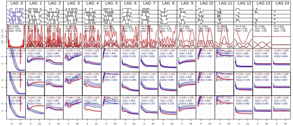
Fig. 3. Evaluation of a randomly chosen 4-code binary sequence of length 15. In the first row of panels the ambiguity functions for each

lag are shown, corresponding to all full lag values. For lag 0 we show the codes themselves (drawn in blue), as the ambiguity functions would be just constants shapes of length equal to the length of the total pulse. The second row of panels shows the average of the squared moduli of the Fourier transforms of the ambiguity over the code set (red) and also the individual terms in this average shown by the darker red lines in bottom. The lower three panels show the behavior of variances of lag profiles if integrated to different resolutions between 1 and 20 baud lengths. The fourth row corresponds to using fractional lags of±2,±1 and 0 to represent each full lag, while in the third row we have used fractional lags±1 and 0 and in the fifth row fractional lags±3,±2,±1 and 0. The red curves in all the rows correspond to a simple calculation using no fractional lags at all, while the blue curves correspond to more realistic analysis, all using the fractional lags specified but 3 different kernels for range integration. The simple red curves are used for fast computer searches and we see that they rather well approximate the more realistic variance estimates.

alternatives are fractional lags±1 and 0 (3rd row), ±2±1 and 0 (4th row) and±3±2±1 and 0 (5th row). If only one row is shown, the fractional lags are±2±1 and 0, which is the most natural choise, as for 5 samples for each baud this results in each fractional lag profile being used once and only once for each full lag profile estimation.

In each of these figures we have plotted in red the simplest possible result for range integration with only full lags taken into account in Eq. (24). This is to make it easy to compare the simple formula to the more careful variance calculations shown by the thick blue, thin blue and dark blue curves cor-responding to more careful calculations, discretized at 1/5 of the baud length and using the different range integration ker-nels defined in Sect. 2.6.

4.4 Normalization of the curves

It is important to understand that we have normalized all the variance curves by dividing them with the number of inde-pendent estimates going into the analysis. These factors in-clude:

– Number of codes in the sequence

– Number of fractional lags

– Range integration

Also, the constantC in Eq. (3) is chosen to be equal to the baud length, so that for the simplest situations – discretized to the baud length – the signal thermal noise is assumed to be of unit variance. In the more accurate calculations discretizing the signal so that each baud corresponds toNflagsamples, the

signal variances are equal toNflagas it should be for sampled

white noise.

The reason for these choises is to make the scales of the different curves comparable. All variances shown in the curves should actually be equal to 1 if they would be calcu-lated by simple estimates just taking into account the number of independent data going to the analysis. The difference from 1 is then a measure of non-perfectness of the inver-sion decoding process and the range-post-integration process caused by correlations of the errors of the inversion process as well as detailed behaviour of the ambiguity functions and the post-integration kernel.

(8)

Index

LAG 0

0.5

1.0

1.5

Index max= 15.00 min= 0.00 R= 0.000 1 2 Index V=1/R= 3003.267 V(1)= 10.469 V(20)= 0.100 1 2 Index V=1/R= 3003.267 V(1)= 5.500 V(20)= 0.110 5 15 1 2 V=1/R= 3003.267 V(1)= 3.562 V(20)= 0.134 Index NULL

LAG 1

Index

NULL

LAG 2

Index

NULL

LAG 3

Index

NULL

LAG 4

Index

NULL

LAG 5

Index

NULL

LAG 6

Index

NULL

LAG 7

Index

NULL

LAG 8

Index

NULL

LAG 9

Index

NULL

[image:8.595.51.549.60.282.2]

max= 1.00 min= 1.00 R= 1.000 Index NULL V=1/R= 1.000 V(1)= 1.108 V(20)= 0.834 Index NULL V=1/R= 1.000 V(1)= 1.195 V(20)= 0.957 5 15 NULL V=1/R= 1.000 V(1)= 1.270 V(20)= 1.052

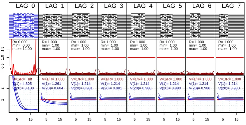
Fig. 4. Evaluation of the chosen code for a 15-baud 4-pulse experiment. While not perfect, the variances as function of range integration

perform significantly better than in the previous figure with a randomly chosen code. For lags 2, 8, 10, 11 and 12 the variances go down faster than the range integration would imply. This is connected with the fact that the Fourier side information curve (red curve in the second row of panels) shows high values for DC and low frequencies.

Index LAG 0

0.5

1.0

1.5

Index max= 12.00 min= 0.00 R= 0.000

5 15

1

2

V=1/R= Inf V(1)= 4.805 V(20)= 0.108

Index

NULL

LAG 1

Index

NULL

max= 1.00 min= 1.00 R= 1.000 5 15 NULL V=1/R= 1.000 V(1)= 1.261 V(20)= 0.604 Index NULL

LAG 2

Index

NULL

LAG 3

Index

NULL

LAG 4

Index

NULL

LAG 5

Index

NULL

LAG 6

Index

NULL

LAG 7

Index

NULL

max= 1.00 min= 1.00 R= 1.000 5 15 NULL V=1/R= 1.000 V(1)= 1.214 V(20)= 0.980

Fig. 5. An alternating code set made from a 16-bit strong alternating code by truncating to 12 bits. We have only shown the most natural

fractional lag set:±2/5,±1/5 and 0. It is clear that all lags≥2 display a perfect decoding behaviour – they behave as if plain 2-pulse pairs corresponding to all 2-pulse-pairs in the set would have been available.

included after simple scalings taking into account the above listed factors are used.

4.5 Numerical data shown in the panes

In the panes we have also helped the inspector by showing some numeric data relevant to the curves. We have shown

[image:8.595.98.500.359.564.2]

(9)

Index LAG 0

0.5

1.0

1.5

Index max= 12.00 min= 0.00 R= 0.000

5 15

1

2

V=1/R= Inf V(1)= 4.805 V(20)= 0.108

Index

NULL

LAG 1

Index

NULL

max= 1.00 min= 1.00 R= 1.000

5 15

NULL

V=1/R= 1.000 V(1)= 1.295 V(20)= 0.554

Index

NULL

LAG 2

Index

NULL

max= 1.00 min= 1.00 R= 1.000

5 15

NULL

V=1/R= 1.000 V(1)= 1.241 V(20)= 0.791

Index

NULL

LAG 3

Index

NULL

max= 1.00 min= 1.00 R= 1.000

5 15

NULL

V=1/R= 1.000 V(1)= 1.249 V(20)= 0.767

Index

NULL

LAG 4

Index

NULL

max= 1.00 min= 1.00 R= 1.000

5 15

NULL

V=1/R= 1.000 V(1)= 1.244 V(20)= 0.802

Index

NULL

LAG 5

Index

NULL

max= 1.00 min= 1.00 R= 1.000

5 15

NULL

V=1/R= 1.000 V(1)= 1.231 V(20)= 0.841

Index

NULL

LAG 6

Index

NULL

max= 1.00 min= 1.00 R= 1.000

5 15

NULL

V=1/R= 1.000 V(1)= 1.233 V(20)= 0.828

Index

NULL

LAG 7

Index

NULL

max= 1.00 min= 1.00 R= 1.000

5 15

NULL

[image:9.595.99.500.62.267.2]

V=1/R= 1.000 V(1)= 1.215 V(20)= 0.941

Fig. 6. A 12-bit weak alternating code set. Some differences to the strong set are visible. While slightly (but insignificantly) worse than the

strong set in case of no range integration, in some cases the integration behaviour is actually better.

Index LAG 0

0.5

1.0

1.5

Index max= 12.00 min= 0.00 R= 0.000

5 15

1

2

V=1/R= Inf V(1)= 4.619 V(20)= 0.107

Index

NULL

LAG 1

Index

NULL

max= 1.00 min= 1.00 R= 1.000

5 15

NULL

V=1/R= 1.000 V(1)= 1.227 V(20)= 0.552

Index

NULL

LAG 2

Index

NULL

max= 1.00 min= 1.00 R= 1.000

5 15

NULL

V=1/R= 1.000 V(1)= 1.209 V(20)= 1.169

Index

NULL

LAG 3

Index

NULL

max= 1.00 min= 1.00 R= 1.000

5 15

NULL

V=1/R= 1.000 V(1)= 1.225 V(20)= 1.259

Index

NULL

LAG 4

Index

NULL

max= 1.00 min= 1.00 R= 1.000

5 15

NULL

V=1/R= 1.000 V(1)= 1.208 V(20)= 1.059

Index

NULL

LAG 5

Index

NULL

max= 1.00 min= 1.00 R= 1.000

5 15

NULL

V=1/R= 1.000 V(1)= 1.181 V(20)= 0.933

Index

NULL

LAG 6

Index

NULL

max= 1.00 min= 1.00 R= 1.000

5 15

NULL

V=1/R= 1.000 V(1)= 1.168 V(20)= 0.978

Index

NULL

LAG 7

Index

NULL

max= 1.00 min= 1.00 R= 1.000

5 15

NULL

V=1/R= 1.000 V(1)= 1.136 V(20)= 0.869

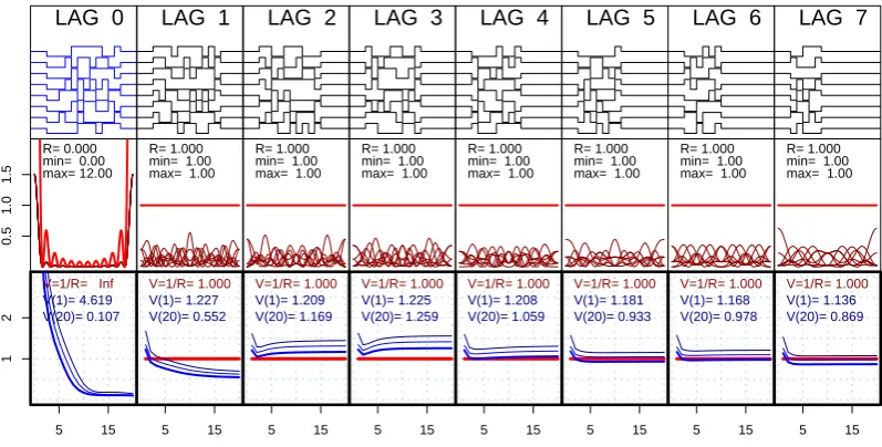
Fig. 7. Alternating code set of length 12 and type 2 introduced by Sulzer. Again the coarse analysis (red curve) represents perfect behaviour,

but it seems that in integration and realistically accurate fractional lag calculations the first lags seem to behave somewhat worse than the alternating codes do.

The inverse ofR,V=1/Rcorresponds to the variance of a normalized situation and we have shown that value on the last rows of panel plotted. The corresponding variance cal-culated more accurately is also shown in dark blue on the same panels, as well as the normalized variance integrated to 1 baud length –V (1)– or to 20 baud lengths –V (20).

5 Interesting behaviour of different alternating codes

[image:9.595.99.498.320.522.2]

(10)

Index LAG 0

0.5

1.0

1.5

Index max= 10.00 min= 0.00 R= 0.000

5 15

1

2

V=1/R= Inf V(1)= 4.375 V(20)= 0.107

Index

NULL

LAG 1

Index

NULL

max= 1.00 min= 1.00 R= 1.000

5 15

NULL

V=1/R= 1.000 V(1)= 1.178 V(20)= 0.470

Index

NULL

LAG 2

Index

NULL

max= 1.00 min= 1.00 R= 1.000

5 15

NULL

V=1/R= 1.000 V(1)= 1.118 V(20)= 0.811

Index

NULL

LAG 3

Index

NULL

max= 1.00 min= 1.00 R= 1.000

5 15

NULL

V=1/R= 1.000 V(1)= 1.111 V(20)= 0.892

Index

NULL

LAG 4

Index

NULL

max= 1.00 min= 1.00 R= 1.000

5 15

NULL

V=1/R= 1.000 V(1)= 1.095 V(20)= 0.897

Index

NULL

LAG 5

Index

NULL

max= 1.00 min= 1.00 R= 1.000

5 15

NULL

V=1/R= 1.000 V(1)= 1.100 V(20)= 0.864

Index

NULL

LAG 6

Index

NULL

max= 1.00 min= 1.00 R= 1.000

5 15

NULL

V=1/R= 1.000 V(1)= 1.104 V(20)= 0.867

Index

NULL

LAG 7

Index

NULL

max= 1.00 min= 1.00 R= 1.000

5 15

NULL

[image:10.595.100.502.60.266.2]

V=1/R= 1.000 V(1)= 1.073 V(20)= 0.796

Fig. 8. Alternating code set of length 10 and type 2. In this set the problem with integration seen in the set of length 12 (previous picture) is

not seen.

Index LAG 0

0.5

1.0

1.5

Index max= 15.00 min= 0.00 R= 0.000

5 15

1

2

V=1/R= 3003.267 V(1)= 5.174 V(20)= 0.098

Index

NULL

LAG 1

Index

NULL

max= 1.74 min= 0.36 R= 0.897

5 15

NULL

V=1/R= 1.115 V(1)= 1.347 V(20)= 0.746

Index

NULL

LAG 2

Index

NULL

max= 1.48 min= 0.47 R= 0.926

5 15

NULL

V=1/R= 1.079 V(1)= 1.277 V(20)= 0.786

Index

NULL

LAG 3

Index

NULL

max= 1.71 min= 0.58 R= 0.938

5 15

NULL

V=1/R= 1.066 V(1)= 1.262 V(20)= 0.597

Index

NULL

LAG 4

Index

NULL

max= 1.41 min= 0.53 R= 0.960

5 15

NULL

V=1/R= 1.042 V(1)= 1.250 V(20)= 1.506

Index

NULL

LAG 5

Index

NULL

max= 1.67 min= 0.50 R= 0.894

5 15

NULL

V=1/R= 1.118 V(1)= 1.341 V(20)= 1.211

Index

NULL

LAG 6

Index

NULL

max= 1.49 min= 0.65 R= 0.943

5 15

NULL

V=1/R= 1.061 V(1)= 1.217 V(20)= 0.706

Index

NULL

LAG 7

Index

NULL

max= 1.53 min= 0.60 R= 0.914

5 15

NULL

V=1/R= 1.094 V(1)= 1.346 V(20)= 1.364

Fig. 9. A set of 15 randomly chosen pulses of 15 bauds each. It seems to be roughly equally good as the chosen set of 4 pulses in Fig. 4.

Very interestingly, weak alternating codes (Fig. 6) may actually perform better in range integration than strong al-ternating codes (Fig. 5). This is because they probably have less phase changes in the ambiguity functions than the strong ones. They are less perfectly similar to independent pulse pairs, and this can actually help regarding integration. For example: a pair of pulses with no phase shift between them behaves better in integration than a single pulse, while of course worse regarding the original resolution.

Type 2 alternating codes of length 12 also show a degrada-tion of performance in range integradegrada-tion (Fig. 7), while those codes of length 10 do not seem to show this (Fig. 8). This

is due to the detailed working of amplitude functions in the sub-baud range resolution, but what exactly happens cannot be explained here.

[image:10.595.97.496.319.521.2]

(11)

[image:11.595.100.501.62.265.2]

Fig. 10. A set of 150 randomly chosen pulses of 15 bauds each. This many pulses are necessary to make random code sets to be comparable

to alternating code sets.

6 Conclusions

We have developed a fast method useful in comparing vari-ances of lag profiles and range-integrated lag profiles using sets of codes in incoherent scatter radar measurements. We have shown that faster and more approximative ways to ap-ply the method produce approximatively the same kinds of results as better modeled and more realistic ways to apply the method. This makes it possible to use the method for ex-tensive computer searches of codes, where speed is essential. We have also shown that the behavior of a new 4-pulse 15-baud code (Fig. 4) is almost as good as known methods of same number of bauds but with much larger number of pulses in the cycle.

In addition, we have found subtle differences in the be-havior of the previously known different types of alternating codes and have seen that randomly chosen code sets need to be very long to produce equally good results as the other methods discussed.

Acknowledgements. This work was supported by the Academy of Finland (application number 213476, Finnish Programme for Cen-tres of Excellence in Research 2006-2011; application number 43988, EISCAT Data Analysis and Research and by the Finnish Graduate School in Astronomy and Space Physics). We are in-debted to Michael Sulzer for suggesting (and practically writing) significant improvements in the introduction.

Topical Editor K. Kauristie thanks M. Lassas and M. Sulzer for their help in evaluating this paper.

References

Damtie, B., Nygr´en, T., Lehtinen, M. S., and Huuskonen, A.: High resolution observations of sporadic-E layers within the polar cap ionosphere using a new incoherent scatter radar experiment,

Ann. Geophys., 20, 1429–1438, 2002, http://www.ann-geophys.net/20/1429/2002/.

Kero, A., Vierinen, J., Enell, C.-F., Virtanen, I., and Turunen, E.: New incoherent scatter diagnostic methods for the heated D-region ionosphere, Ann. Geophys., in press, 2008.

Lehtinen, M., Damtie, B., and Nygr´en, T.: Optimal binary phase codes and sidelobe-free decoding filters with application to inco-herent scatter radar, Ann. Geophys., 22, 1623–1632, 2004, http://www.ann-geophys.net/22/1623/2004/.

Lehtinen, M. S.: Statistical theory of incoherent scatter radar mea-surements, Ph.D. thesis, University of Helsinki, 1986.

Lehtinen, M. S. and H¨aggstrom, I.: A new modulation principle for incoherent scatter measurements, Radio Sci., 22, 625–634, 1987. Lehtinen, M. S. and Huuskonen, A.: General incoherent scatter analysis and GUISDAP, J. Atmos. Terr. Phys., 58, 435–452, 1996.

Markkanen, M., Vierinen, J., and Markkanen, J.: Polyphase alter-nating codes, Ann. Geophys., 26, 2237–2243, 2008,

http://www.ann-geophys.net/26/2237/2008/.

Sulzer, M. P.: A new type of alternating code for incoherent scatter measurements, Radio Sci., 28, 995–1002, 1993.

Vierinen, J., Lehtinen, M., Orisp¨a¨a, M., and Virtanen, I.: Transmis-sion code optimization method for incoherent scatter radar, Ann. Geophys., accepted, 2008a.

Vierinen, J., Lehtinen, M., and Virtanen, I.: Amplitude domain analysis of strong range and Doppler spread radar echos, Ann. Geophys., in press, 2008b.

Virtanen, I. I., Lehtinen, M. S., Nygrén, T., Orispää, M., and Vieri-nen, J.: Lag profile inversion method for EISCAT data analysis, Ann. Geophys., 26, 571–581, 2007,

http://www.ann-geophys.net/26/571/2007/.