SRef-ID: 1432-0576/ag/2005-23-909 © European Geosciences Union 2005
Annales
Geophysicae
The role of 3-D geomagnetic induction in the determination of the
ionospheric currents from the ground geomagnetic data
A. Pulkkinen1and M. Engels2
1NASA/GSFC, Greenbelt, Code 692, MD 20770, USA
2Federal Institute for Geosciences and Natural Resources, Stilleweg 2, 30655 Hannover, Germany
Received: 25 August 2004 – Revised: 13 January 2005 – Accepted: 27 January 2005 – Published: 30 March 2005
Abstract. The geomagnetic field variations measured at the
surface of the Earth are composed of both internal and ex-ternal parts. The exex-ternal field arises from the sources in the magnetosphere and ionosphere, whereas the internal field is generated by the currents induced within the Earth. The in-ternal part may in some situations comprise a notable part of the measured total field and thus a blind usage of geomag-netic field recordings potentially produces significant errors to estimated ionospheric currents. In this paper the role of ge-omagnetic induction in auroral ionospheric studies is inves-tigated by modeling the induction using simultaneously the realistic ionospheric source and a realistic three-dimensional Earth conductivity structure.
The modeling results imply that the effects of the lat-eral ground conductivity anomalies on ionospheric equiva-lent current patterns are, though clearly detected, less severe than anticipated for fields varying with periods from 5 to 120 min. However, the amplification of the determined cur-rents caused by induction is significant, leading to an over-estimation of up to 30% of the main current flow intensi-ties, with the overestimation increasing sharply when moving away from the region of the main flow.
In addition to the 3-D modeling, a simple method is intro-duced to help estimate the internal contribution to the mea-sured variations of theI Lindex (local variant of theAL in-dex). A test with the 26 June 1998 substorm event indicates that the method can help to extract the internal contribution from theI Lindex.
Keywords. Geomagnetism and paleomagnetism
(Geomag-netic induction)
1 Introduction
The magnetic effect arising from electromagnetic induction inside the Earth contributes to the total magnetic field mea-sured at the surface of the Earth. Depending on the indi-Correspondence to: A. Pulkkinen
vidual situation and the accuracy with which the conclusions are drawn from the data, it may be acceptable to disregard the internal effects. For example, in ionospheric studies the effects of the induction are often neglected. Studies where the internal effects are negligible include, in particular, in-vestigations of temporally relatively steady current systems that do not induce notable currents in the Earth - induction is a time dependent phenomenon. However, when more dy-namic situations are concerned, neglecting the induction may lead to erroneous interpretations. In some cases, for exam-ple in particular solid Earth studies, separated field compo-nents are needed as a starting point for the entire investigation (e.g. Berdichevsky and Zhdanov, 1984, p. 191). Earlier in-vestigations have shown that neglecting telluric effects may cause significant errors of up to 40% in the estimation of the ionospheric current intensity (Viljanen et al., 1995; Tanska-nen et al., 2001), or even notable errors in the determination of some global magnetospheric indices likeDst (H¨akkinen et al., 2002). As finer spatial and temporal scales are inves-tigated both in ionospheric and magnetospheric studies and more accurate estimates of the physical parameters are pur-sued, errors of 40% become significant and cannot be blindly neglected. It is thus clear that geomagnetic induction should be taken into account in detailed studies of ionospheric and magnetospheric dynamics and further understanding of the distorting effects of geomagnetic induction, especially in re-gions with strong conductivity gradients, is needed.
25 oW
0
o
25
o
E
50 o E 75
o E
54o N
60o
N 66o
N 72
o N
[image:2.595.50.285.65.298.2]78 o N
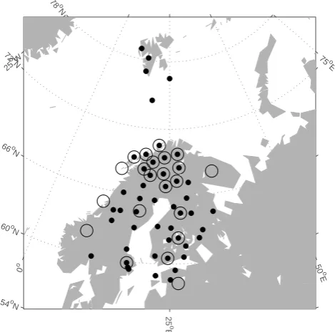
Fig. 1. Location of magnetometer sites used for the derivation of the original source currents (black dots) and the location of sites used for the derivation of the currents used in the comparison (circles). Geographic coordinates are used.
01:00 02:00 03:00 04:00 05:00 06:00 07:00 −1200
−1000 −800 −600 −400 −200 0
UT [h]
[image:2.595.51.286.371.555.2]IL [nT]
Fig. 2. The local variant ofAL,I Lindex computed from the mea-sured IMAGE magnetometer array data for 26 June 1998. The dashed lines indicate 01:00 UT and 03:00 UT, respectively.
and Baumjohann, 1993) and the non-one-dimensional na-ture of the Earth’s crust (e.g. Heinson, 1999, and references therein), the approximations seem quite crude, thus impos-ing limitations to the conclusions drawn from these earlier investigations. Here, for the first time, a realistic three-dimensional (3-D) model of the ground conductivity is com-bined with a geometrically varying and arbitrarily moving re-alistic ionospheric source. Comparisons between the original ionospheric source and the ionospheric source deduced using the ground magnetic field “contaminated” by the modeled
induction enables us to estimate the effect of the induction more realistically than in earlier investigations. Olsen and Kuvshinov (2004) have used a similar approach to study the coast effect of geomagnetic storms, i.e. a global conductivity model was excited with magnetic field variations produced by the ring current. Their study, however, due to its global nature, is not directly comparable to the regional study car-ried out here.
In Sect. 2, we describe the modeling procedure that en-ables the combination of the 2-D ionospheric source and 3-D geomagnetic induction. In Sect. 3, we carry out a detailed analysis of the modeled data and the impact of 3-D induc-tion on the determined ionospheric equivalent currents is es-timated. Also, a new, simple method for estimating the inter-nal effects on geomagnetic indices, likeI L(the local variant of theALindex computed from the IMAGE magnetometer array data; see Kauristie et al. (1996)), is introduced. The theoretical basis of the method is given in the Appendix. Fi-nally, in Sect. 4, summary and concluding remarks with gen-eral implications of the study are given.
2 Modeling procedure
A volume-3-D induction code by Avdeev et al. (2002), com-bined with the new field separation technique introduced by Pulkkinen et al. (2003b), provide efficient tools for the treat-ment given in the paper. The four-step modeling procedure is as follows:
1. Data from the Baltic Electromagnetic Array Research (BEAR) project during which both the electric and mag-netic field were recorded in a dense array covering Fennoscandia (Korja et al., 2002), combined with IM-AGE magnetometer array data, are used (black dots in Fig. 1). First, the geomagnetic data are separated into internal and external parts to obtain the best possible es-timate of the ionospheric equivalent source (Pulkkinen et al., 2003b).
Fig. 3. Log10of the average taken over the Fennoscandian crustal (0–60 km) conductivity [S/m] model used in the volume-3-D induc-tion code.
construction of the 3-D model is also described in de-tail. Modeling frequencies are 24 harmonics of the se-lected two-hour event, resulting in a period range from 5 to 120 min. All model cells have a 20-km base length and the total modeling area extends to 168×180 cells (3360 km×3600 km), surrounded by the 1-D normal section.
3. The output of the modeling code consists of the elec-tromagnetic fields for each modeling cell in frequency domain. After inverse Fourier transformation back into time domain, two magnetic data sets are extracted for the continental IMAGE magnetometer locations (circles in Fig. 1): one with the total and another with the exter-nal part of the magnetic field. The northernmost IM-AGE sites are not applicable due to their vicinity to the volume-3-D modeling boundary.
4. From the two sets of magnetic field data, we derive two sets of ionospheric equivalent currents (on equiva-lent currents, see e.g., Untiedt and Baumjohann, 1993), using the spherical elementary current system method (Amm and Viljanen, 1999; Pulkkinen et al., 2003a). The currents are derived to 110 km height. Only the horizon-tal components of the magnetic field are used. This is due to the fact that the horizontal field can always be explained by a source only in the ionosphere, or in the ground (for a more detailed discussion, see Pulkkinen et al., 2003a). Thus, the vertical component of the mag-netic field is not treated in this investigation. Finally, the difference between the two sets of equivalent currents is analyzed and the impact of induction in the ground on the equivalent currents is estimated.
std(EX), max 892 mV/km
0 o
12
o E
24
o
E
36
o E
48
o
E
56o
N
60o
N
64o
N
68o
N 72o
N
std(EY), max 906 mV/km
0 o
12
o E
24
o
E
36
o E
48
o
E
56o
N
60o
N
64o
N
68o
N 72o
N
std(EX), max 892 mV/km
0 o
12
o E
24
o
E
36
o E
48
o
E
56o
N
60o
N
64o
N
68o
N 72o
N std(EY), max 906 mV/km
0 o
12
o E
24
o
E
36
o E
48
o
E
56o
N
60o
N
64o
N
68o
N 72o
N
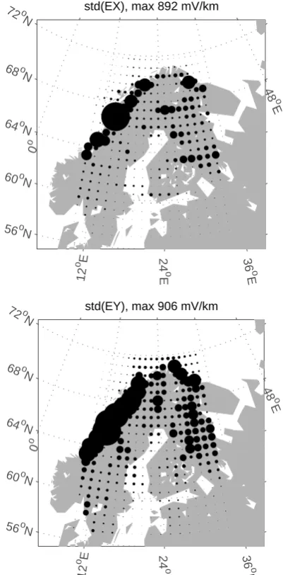
Fig. 4. Standard deviation of the modeled geoelectric field varia-tions at the Earth’s surface at some of the grid points of the volume-3-D code. The maximum standard deviations are indicated in the titles of the figures.
3 Analysis
[image:3.595.49.290.63.259.2]Modeled std(Htot),std(Hext), max 357.9 nT, 261.6 nT
0
o
12 o E
24
o
E
36
o E
48
o
E
56o
N
60o
N
64o
N
68o
N 72o
N Measured std(H), max 359.6 nT
0
o
12 o E
24
o
E
36
o E
48
o
E
56o
N
60o
N
64o
N
68o
N 72o
N
Modeled std(Htot),std(Hext), max 357.9 nT, 261.6 nT
0 o
12
o E
24
o
E
36
o E
48
o
E
56o
N
60o
N
64o
N
68o
N 72o
N
Measured std(H), max 359.6 nT
0 o
12
o E
24
o
E
36
o E
48
o
E
56o
N
60o
N
64o
N
68o
N 72o
N
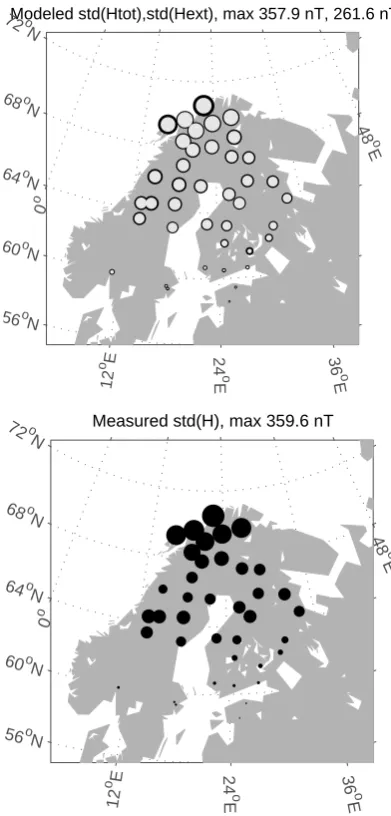
Fig. 5. Standard deviations of the modeled and the measured hori-zontal magnetic field variations. Light and black circles on the top panel correspond to standard deviations of the external field and the total field, respectively. The maximum standard deviations are indi-cated in the titles of the figures.
the ground. Figure 5, in turn, shows the modeled and mea-sured standard deviations of the horizontal magnetic field. The measured data was low-pass filtered to contain only pe-riods of 5 min and above, to correspond to the pepe-riods in-cluded in the modeled data. It is seen that the magnitudes of the standard deviations and the spatial patterns of the to-tal modeled and the measured field variations coincide very well with each other. Furthermore, as seen by comparing the external and the total modeled magnetic field variations, induced fields amplify the external field variations, as ex-pected. Finally, as can be verified by comparing Figs. 6 and 13, the modeled and the measured 5-min low-pass filteredI L index, respectively, the modeledI Lcoincides well with the measurements, yet there is another indication of a realistic Earth response. Thus, it can be concluded that the modeling
20 30 40 50 60 70 80 90 100
−1000 −800 −600 −400 −200 0
Time [min]
IL [nT]
20 30 40 50 60 70 80 90 100
70 75 80 85 90
Time [min]
ILext
/IL
tot
[image:4.595.66.262.61.470.2][%]
Fig. 6. Top panel: modeled external (dashed), internal (thin solid) and the totalI L(thick solid) index. bottom panel: ratio between the externalI Land the totalI L. time is minutes from the beginning of the modeling period of 26 June 1998, 01:00 UT. The dashed line indicates the time 01:55 UT.
procedure produces both 3-D and an realistic Earth response, and thus the modeled fields can be assumed to reflect the true characteristics of the investigated phenomenon.
[image:4.595.313.545.64.245.2]Equi. ext., max 1439.0 mA/m
0 o
12 oE
24
o
E
36
o E
48 o E
56oN
60o
N
64o
N
68oN
72o
[image:5.595.329.525.63.263.2]N
Fig. 7. Ionospheric equivalent currents (Jext) determined from the external part of the modeled magnetic field. Magnetic field data from the continental IMAGE array locations for time 01:55 UT are used (see Fig. 6). The maximum current amplitude is indicated in the title of the figure.
Equi. tot., max 2021.1 mA/m
0 o
12
oE
24
o
E
36
o
E 48
o
E
56oN
60o
N
64o
N
68o
N 72
oN
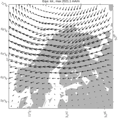
Fig. 8. Ionospheric equivalent currents (Jt ot) determined from the total modeled magnetic field. Magnetic field data from the con-tinental IMAGE array locations for time 01:55 UT are used (see Fig. 6). The maximum current amplitude is indicated in the title of the figure.
the asthenosphere variant with an increased conductance at 200–300 km depth would enhance the internal contribution on the order of 5–10%. However, the usage of a slightly too resistive conductivity model does not affect the basic conclu-sions of the study.
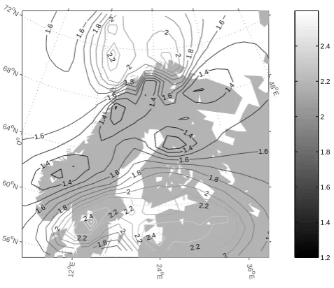
In Figs. 7−10 we show a snapshot of the derived iono-spheric equivalent currents and their relative differences for the time when the peak internal contribution toI Loccurs.
Equi. diff.(int.), max 667.9 mA/m
0 o
12 oE
24
o
E
36
o E
48 o E
56oN
60o
N
64o
N
68o
N
72o
[image:5.595.68.265.65.263.2]N
Fig. 9. Difference between the ionospheric equivalent currents de-termined from the total and external parts of the modeled magnetic field. Magnetic field data from the continental IMAGE array loca-tions for time 01:55 UT are used (see Fig. 6). The maximum current amplitude (difference) is indicated in the title of the figure.
0 o
12
oE
24
o
E
36
o
E 48
o
E
56o
N
60o
N
64oN
68o
N
72o
N
11.2
1.4 1.4
1.4
1.4
1.4
1.4 1.4
1.4
1.4 1.6
1.6
1.6
1.6
1.6
1.6 1.6 1.6
1.6
1.6
1.6
1.8
1.8
1.8
1.8 1.8
1.8
1.8
2
2
2
2
2
2
2
2
2.2
2.2 2.2 2.2
2.2
2.2
2.2
2.4 2.4
2.4
2.4
2.4
2.4
2.6
2.6 2.6
2.6
2.6
2.8 2.8
2.8
3
1 1.2 1.4 1.6 1.8 2 2.2 2.4 2.6 2.8 3
Fig. 10. Log10 of the relative difference 100·|Jt ot−Jext|/|Jext|. See Figs. 7−9.
[image:5.595.306.546.347.547.2] [image:5.595.67.267.352.552.2]0 o
12
oE
24
o
E
36
o
E 48
o
E
56o
N
60o
N
64o
N
68o
N
72o
N
1.4
1.4
1.4
1.4
1.4
1.4
1.4
1.4 1.6
1.6 1.6
1.6 1.6
1.6
1.6 1.6
1.6
1.6
1.8
1.8 1.8
1.8
1.8
1.8 1.8
1.8 2
2
2
2
2 2
2 2
2
2.2 2.2
2.2
2.2
2.2 2.2 2.2
2.4 2.4
1.2 1.4 1.6 1.8 2 2.2 2.4
Fig. 11. Log10 of the mean relative difference 100·|Jt ot−Jext|/|Jext|taken over the entire modeling period.
101 102
102 103
Period [min]
[image:6.595.48.287.61.267.2]Penetration depth [km]
Fig. 12. Penetration depth of the periods from 5 to 120 min for aver-age conductivities in Fig. 3. Thin lines correspond to conductivities 10−0.5,10−1.5,10−2.5and 10−3.5S/m from the bottom to the top. The thick line indicates the 60 km penetration depth, i.e. the bottom of the 3-D crust used in the modeling.
as rapidly as that of the ionospheric currents (for a more de-tailed discussion on this see, e.g. Tanskanen et al., 2001). Varentsov et al. (2002) found strong electromagnetic sound-ing parameter-related distortions caused by the same 3-D crust model. Thus, it is surprising that the overall equiva-lent current pattern is not very severely distorted in the re-gion of the main current flow, i.e. gradients in Fig. 10 are relatively small. There are, however, features that clearly re-late to inhomogeneities of the model, for example, the band of conductivity enhancement through the center parts of the model, as well as the currents induced in a well-conducting sea channel, as seen from Figs. 9 and 10. Also, the patch
of the conductivity enhancement in northern Fennoscandia clearly creates distortions to the equivalent current patterns.
Features observed in Figs. 7−10 are also reproduced in the mean behavior of the relative difference taken over the whole modeling period depicted in Fig. 11. Excluding the impact of the complex 3-D structures in northern Fennoscan-dia, which cause some observable distortions even under the main current flow, the pattern-distorting effects of conduc-tivity anomalies are seen even less in the mean values. The regions with a large relative difference correspond mainly to areas where the mean current amplitude is small. It is thus clear that for the investigated periods (5 to 120 min), the strong inhomogeneities in the crust (0–60 km) affect the basic equivalent patterns relatively little, even during very dynamic events such as substorms.
The reason for the small effect of the 3-D crust structures is that the electromagnetic field, especially for the lower fre-quency portion of the external variations that comprise the majority of the observed signal, penetrates to depths greater than 60 km. At these depths, in terms of the horizontal con-ductivity variations, the smoother upper mantle creates a spa-tially smooth response in the surface geomagnetic field. This is illustrated in Fig. 12, where the penetration depths for av-erage conductivities of Fig. 3 for periods used in the mod-eling are shown. The light shading indicates the portion of the field penetrating below 60 km, i.e. to depths having 1-D conductivity, where dark shading, in turn, indicates the portion penetrating to less than 60 km. As seen, the major part of the relatively low-frequency source field created by the varying ionospheric equivalent currents does not “see” the upper crust inhomogeneities because of the large depth to which it penetrates. Thus, spatially smooth induced fields are to follow. Furthermore, in comparison to the geoelectric response, the geomagnetic response “integrates” information from larger areas. This results in smoother overall field pat-terns, as seen by comparing Figs. 4 and 5.
Based on the findings above, it is clear that in most of the ionospheric investigations the amplification of the deter-mined current amplitudes, due to geomagnetic induction, is probably a more severe problem than the actual spatial dis-tortion of the computed current patterns. This and the wide use of different indices derived from geomagnetic recordings encouraged us to seek a useful relation that could be used in estimating the internal part, for example, of the measuredI L index. The details of deriving such a relation are given in the Appendix; the final result is
I Lint(ω)=I Lt ot(ω) α
2(α+p), (1)
whereI Lt ot is the measured signal,α=h+Lis the sum of the heighthand 2Lhalf-width of the electrojet. For a homo-geneous Earth we have
p=√ 1
iωµ0σ
, (2)
[image:6.595.50.286.315.506.2]transform the measured signal, carry out the multiplication and invert the internal part back to the time domain.
Let us make a few observations from Eq. (1) that character-ize some of the very basic features of geomagnetic induction. First, as the conductivity increases, the internal part also in-creases: for a perfectly conducting Earth, the internal part is exactly half of the measured signal. Secondly, the increas-ing width of the electrojet also increases the internal part: for α|p|, i.e. the source is planar, the internal part is again ex-actly half of the measured signal. Obviously, withω=0 there is no induction in the Earth and the internal part vanishes.
[image:7.595.310.546.61.240.2]To test the new method, we separated the measured, 5-min low-pass filteredI Lindex for the 26 June 1998 event. An effective conductivity of 10−2S/m (and for comparison with conductivities 10−1S/m and 10−3S/m) andαof 610 km were used. The choices are good estimates for the present situation, as can be verified from Figs. 3 and 7. To have the best possible correspondence with Fig. 6, only the con-tinental IMAGE stations were used. The result is shown in Fig. 13. The similarity with Fig. 6 is clear: after the onset of the substorm, the internal part increases, reaches its max-imum of about 30% at the end of the expansion phase after which a gradual decrease follows. Thus, although a more thorough analysis of the performance of Eq. (1) is needed, the simple method seems to produce a very realistic internal field for the 26 June 1998 substorm period. However, keep-ing the approximations made in derivkeep-ing Eq. (1) in mind it should be emphasized that a reliable estimation of the inter-nal part from the measured magnetic field variations requires 2-D array data and the application of rigorous magnetic field separation methods (see Pulkkinen et al., 2003b).
4 Conclusions
In this investigation, a combination of a field separation tech-nique (Pulkkinen et al., 2003b) with a volume-3-D modeling of geomagnetic induction (Avdeev et al., 2002) was intro-duced. The combination was applied using a unique data set of geomagnetic recordings and a realistic model of the Earth’s 3-D conductivity (Korja et al., 2002). The model-ing results were used to study the impact of induction in the Fennoscandian region on the auroral ionospheric currents de-termined from the geomagnetic field recordings.
It was seen that despite the strong 3-D anomalies con-tained in the conductivity model, the overall spatial patterns of the determined ionospheric equivalent currents were not severely distorted. Although the effects of the 3-D induction were identified, the majority of the induced currents (for peri-ods from 5 to 120 min) flowed in the depths below the strong crustal conductivity anomalies, thus resulting in spatially rel-atively smooth, magnetic field variations. However, despite the small spatial effects of the 3-D conductivity, otherwise significant induction effects were observed. During the stud-ied substorm onset, the amplitude of the current was overes-timated by about 30%. This is a number which can certainly affect, for example, estimations of the total ionospheric Joule
01:00 01:15 01:30 01:45 02:00 02:15 02:30 02:45 03:00
−1200 −1000 −800 −600 −400 −200 0
UT [h]
IL [nT]
01:00 01:15 01:30 01:45 02:00 02:15 02:30 02:45 03:00
60 70 80 90 100
UT [h] ILext
/IL
tot
[%]
01:00 01:15 01:30 01:45 02:00 02:15 02:30 02:45 03:00 −1200
−1000 −800 −600 −400 −200 0
UT [h]
IL [nT]
01:00 01:15 01:30 01:45 02:00 02:15 02:30 02:45 03:00 60
70 80 90 100
UT [h]
ILext
/IL
tot
[%]
Fig. 13. Top panel: the measured total (thick solid) and the com-puted internal part of the 5-min low-pass filteredI Lindex for the 26 June 1998 substorm event. Bottom panel: ratio between the external
I Land the totalI L. Only continental IMAGE stations were used to compute the index. The dashed curves in both panels correspond to fields computed with conductivities 10−1S/m (lower curve) and 10−3S/m (upper curve), respectively. See the text for details.
heating and thus may also impact the estimations of the total magnetospheric energy budget (e.g. Tanskanen, 2002). Fur-thermore, the rapid increase of the internal part relative to the total magnetic field when moving away from the main iono-spheric current flow was underscored. Accordingly, special care should be taken when interpreting data outside the main flow. In summary, though the spatial effects were found to be smaller than anticipated, it is clear that geomagnetic in-duction should be taken into account in detailed ionospheric investigations.
It should be noted that the conclusions made here are strictly applicable only for the source used and the conduc-tivity model used, generalizations to other situations should be made with care. For example, the well-conducting sea is rather shallow in the western coast of Fennoscandia; steeper boundaries between deep seas and continents are more likely to also distort the spatial patterns of the computed iono-spheric equivalent currents. Likewise, the study is strictly valid only for periods used of the field variations, i.e. periods from 5 to 120 min. The higher-frequency electromagnetic fields which do not penetrate as deep may be distorted more severely by the 3-D conductivity anomalies in the crust. If the high-frequency component is not critical for a specific study, it may be worthwhile to low-pass filter the data to contain only frequencies that can be assumed to penetrate in the ground down to depths with smoother conductivity vari-ations.
in the derivation of the relation, application to IMAGE ar-ray geomagnetic data of the 26 June 1998 substorm event produced very reasonable results. Thus, especially under a well-defined, one-dimensional electrojet (no significant vari-ations in they-direction), with good approximate estimates of the effective ground conductivity and the electrojet width, the method can significantly improve the estimates of the ex-ternal part in theI Lindex variations.
Appendix A
Here the derivation of Eq. (1) is presented. The setting is as follows: 1. We assume a one-dimensional, infinitely long electrojet at heighthhaving current distribution with the flow to they-direction given by
jy(x)= I
π L
x2+L2, (A1)
where I is the current amplitude and 2L is the half-width of the distribution. The magnetic field at the Earth’s surface produced by the distribution in Eq. (A1) is equal to the field of a line current at heighth+L(Maurer and Theile, 1978). 2. We assume a homogeneous Earth with conductivityσ, and as usually in geomagnetic investigations, variations are assumed to be slow enough to justify the neglect of the dis-placement currents.
Using the complex image method, which is an extension of a classical method of images (e.g. Jackson, 1999, p.57), for an infinitely long line current (Boteler and Pirjola, 1998), we obtain an expression for the total magnetic field at the surface of the Earth directly below the line current (x=0)
Bxt ot(x=0)= µ0I
2π
1
α + 1 α+2p,
, (A2)
where α=h+L and p represent the complex depth of the image current which reduces for a homogeneous Earth to (Schmucker, 1970)
p=√ 1
iωµ0σ
(A3) whereωandµ0are the angular frequency (2πf) of the vari-ations and the vacuum permeability, respectively. Note that Eq. (A2) is valid for any layered Earth conductivity, if a gen-eral definition of the complex depth is used. The complex im-age approximation is generally valid when|pv|31 wherev is the wave number of the horizontal field variations (Thom-son and Weaver, 1975; Boteler and Pirjola, 1998).
Now, the second term in the right-hand side of Eq. (A2) corresponds to the internal component produced by the im-age current at depth h+L+2p, and thus the ratio between the internal and the total components of the magnetic field can be expressed as
Bxint Bt ot x
= α
2(α+p). (A4)
The I L index is supposed, by definition, to measure the maximum excursion of the x-component of the magnetic field from the baseline level. Accordingly, if we assume a 1-D electrojet as described above, the value enteringI L is obtained directly below the center of the electrojet, i.e. I Lt ot=Bxt ot(x=0). Thus, we may interchange the two to give in the frequency domain
I Lint(ω)=I Lt ot(ω) α
2(α+p) (A5)
which is the result we were looking for.
Acknowledgements. The research was performed while AP held a National Research Council Associateship Award at NASA/Goddard Space Flight Center. This investigation could not have been made without the great efforts of the BEAR project team responsible for part of the data used in the study at hand. The project was a good demonstration of how the knowledge coming from both the space physics and the solid earth communities can be combined for a new science. Invaluable comments by A. Viljanen and two referees on the manuscript are greatly acknowledged.
The Editor in Chief thanks A. Kuvshinov and another referee for their help in evaluating this paper.
References
Amm, O. and Viljanen, A.: Ionospheric disturbance magnetic field continuation from the ground to ionosphere using spherical ele-mentary current systems, Earth, Planets and Space, 51, 431–440, 1999.
Avdeev, D. B., Kuvshinov, A. V., Pankratov, O. V., and Newman, O. G.: Three-dimensional induction logging problems , Part I: An integral eqution solution and model comparisons, Geophysics, 67(2), 413–426, 2002.
Beamish D., Clark, T. D. G., Clarke, E., and Thomson, A. W. P.: Geomagnetically induced currents in the UK: geomagnetic vari-ations and surface electric fields. J. Atmos. Sol. Terr. Phys, 64, 1779–1792, 2002.
Berdichevsky, M. and Zhdanov, M,: Advanced theory of deep ge-omagnetic sounding, Elsevier Science Publishers B. V., Nether-lands, 408, 1984.
Boteler, D. H. and Pirjola, R. J.: The complex-image method for calculating the magnetic and electric fields produced at the sur-face of the Earth by the auroral electrojet, Geophys. J. Int., 132(1), 31–40, 1998.
Engels, M., Korja, T., and BEAR Working Group: Multisheet mod-elling of the electrical conductivity structure in the Fennoscan-dian Shield, Earth Planets Space, 54, 559–573, 2002.
Heinson, G.: Electromagnetic studies of the lithosphere and as-thenosphere, Surv. Geophys., 20, 229–255, 1999.
H¨akkinen, L., Pulkkinen, T. I., Nevanlinna, H., Pirjola, R., and Tanskanen, E: Effects of induced currents onDst and on mag-netic variations at mid-latitude stations, J. Geophys. Res., 107, doi:10.1029/2001JA900130, 2002.
Jackson, D.: Classical Electrodynamics, 3rd ed., John Wiley and Sons, Inc., 1999.
Kamide, Y. and Baumjohann, W.: Magnetosphere-ionosphere cou-pling, Physics and Chemistry in Space, 23, 178, 1993.
Kauristie, K., Pulkkinen, T. I., Pellinen, R. J., and Opgenoorth, H. J.: What can we tell about global auroral electrojet activity from a single meridional magnetometer chain?, Ann. Geophys., 14, 1177–1185, 1996,
http://direct.sref.org/1432-0576/ag/1996-14-1177 SRef-ID: 1432-0576/ag/1996-14-1177.
Korja, T., Engels, M., Zhamaletdinov, A. A., Kovtun, A. A., Palshin, N. A., Smirnov, M. Yu., Tokarev, A., Asming, V. E., Vanyan, L. L., Vardaniants I. L., and the BEAR Working Group: Crustal conductivity in Fennoscandia - a compilation of a database on crustal conductance in the Fennoscandian Shield, Earth, Planets and Space, 54, 535–558, 2002.
Mareschal, M.: Modelling of natural sources of magnetospheric ori-gin in the interpretation of regional induction studies: a review, Surveys in Geophysics, 8, 261–300, 1986.
Maurer, H. and Theile, B.: Parameters of the Auroral Electrojet From Magnetic Variations Along a Meridian. J. Geophys., 44, 415–426, 1978.
Olsen, N. and Kuvshinov, A.: Modeling the ocean effect of geo-magnetic storms, Earth Planets Space, 56, 525–530, 2004. Pirjola, R.: Electromagnetic induction in the Earth by a plane wave
or by fields of line currents harmonic in time and space, Geo-physica, 18, 1982.
Pulkkinen, A., Amm, O., Viljanen, A., and BEAR Working Group: Ionospheric equivalent current distributions determined with the method of spherical elementary current systems, J. Geophys. Res., 108, doi:10.1029/2001JA005085, 2003a.
Pulkkinen, A., Amm, O., Viljanen, A., and BEAR Working Group: Separation of the geomagnetic variation field on the ground into external and internal parts using the spherical elementary current system method, Earth, Planets and Space, 55, 117–129, 2003b. Schmucker, U.: Anomalies of geomagnetic variations in the
southwestern United States, 13., Bull. Scripps, Institution of Oceanographie, University of California, 1970.
Tanskanen, E. I., Viljanen, A., Pulkkinen, T. I., Pirjola, R., H¨akkinen, L., Pulkkinen, A., and Amm, O.: At substorm on-set, 40% of AL comes from underground, J. Geophys. Res., 106, 13 119–13 134, 2001.
Tanskanen, E.: Terrestrial substorms as a part of global energy flow, PhD thesis, Finnish Meteorological Institute, Contributions, 36, 2002.
Thomson, D. J. and Weaver, J. T.: The complex image approxima-tion for inducapproxima-tion in a multilayered Earth, J. Geophys. Res., 80, 123–129, 1975.
Untiedt, J. and Baumjohann, W.: Studies of polar current systems using the IMS Scandinavian magnetometer array, Space Sci. Rev., 63, 245–390, 1993.
Varentsov, I., Engels, M., Korja, T., Smirnov, M., and the BEAR Working Group: A generalized model of Fennoscandia: a chal-lenging database for long-period 3-D modeling studies within the Baltic Electromagnetic Array Research (BEAR) project, Izvestija, Phys. Solid Earth, 38, 855–896, 2002.
Viljanen, A., Kauristie, K., and Pajunp¨a¨a, K.: On induction effects at EISCAT and IMAGE magnetometer stations, Geophys. J. Int., 121, 893–906, 1995.