Numerical Analysis of In-Cylinder Flow in Internal Combustion Engines by LES Method

AUT J. Mech. Eng., 1(1) (2017) 29-38 DOI: 10.22060/mej.2016.748

Numerical Analysis of In-Cylinder Flow in Internal Combustion Engines by LES

Method

M. Khorramdel, H. Khaleghi*_{, Gh. Heidarinejad, M. H. Saberi} Department of Mechanical Engineering, Tarbiat Modares University, Tehran, Iran

ABSTRACT: In this research, Large Eddy Simulation of in-cylinder flow during suction and compression stroke in an axisymmetric engine is performed. A computer code using Smogorinsky subgrid model is developed to solve the governing equations of the flow. A proper understanding of flow during suction and compression strokes, gives better information for fuel/air mixture and combustion. The results show that the advantage of LES model is the ability of computing turbulence characteristics in various crank angles of engine cycle. This advantage of model is highlighted by calculating RMS values of axial velocity in comparison with experimental ones. The results show that axial velocity fluctuations during intake reaches to a higher level than in compression stroke because of the inlet jet to the cylinder and intensive gradient of variables. In this regard, the flow in 100 degree ATDC during intake stroke reaches the maximum level of turbulence intensity and then turbulence generated during intake stroke decays rapidly. During intake stroke, three main vorticities are generated inside the cylinder. In the compression stroke these three vorticities are merged together to establish a new vorticity with direction of rotation opposite to the intake flow. Some smaller recirculating regions are also generated at 90 degree BTDC.

Review History:

Received: 18 February 2016 Revised: 14 May 2016 Accepted: 29 May 2016

Available Online: 8 November 2016

Keywords:

Internal combustion engines In-cylinder flow

Large eddy simulation Crank angle

1- Introduction

The simulation of actual behavior and study of the mixing and combustion phenomena in internal combustion engines

depend on reliable forecasts of turbulence in the intake and compression stroke. During suction stroke in a diesel

engine, the air flow in the manifold moves into the cylinder

by passing through the entrance valve. When the air is

passing through the inlet valve, a jet flow will be created. The geometrical configuration of the inlet valve and its movement schedule will perform an organized pattern of flow named swirl motion (circulation around cylinder’s axis) and tumble motion (circulation perpendicular to cylinder’s axis). The

most of the energy from inlet flow will be converted to the

turbulence in the suction stroke.

During investigations, it was found that in-cylinder flow

field at the end of the compression stroke and before an

injection of the fuel, has a significant impact on improving

air-fuel mixing as well as the combustion process that can

provide valuable design information to engineers. For this reason, the importance of identifying and studying the flow

in the intake and compression stroke in recent years has been

attracted great attention and wide range of investigations

have been made by using numerical and experimental methods.

In turbulence field, during recent decades, several turbulence models have been used to simulate the flow field in internal

combustion engines by researchers. They obtained relatively

successful results using the turbulence model based on

Reynolds Averaged Navier-stokes (RANS). Among these

simulations, Mosleh and Khaleghi [1] simulated the

in-cylinder flow in an Internal Combustion Engine (ICE) using

k-ε model. Their simulation was on a symmetric combustion

chamber. Comparison of SIMPLE and PISO algorithms for intake flow was one of the main results of their simulation

and they found that both algorithms have appropriate performances

in the calculations. Also, they obtained very good results compared to experimental data. Fallah and Khaleghi [2]

simulated the fluid flow in reciprocating engines using k-ε and ASM turbulence models. They compared these two turbulence models and found that ASM model was more

accurate in calculating the flow characteristics compared to

the K-ε model.

In fact, the contribution of these turbulence models in

ICE industry progress cannot be ignored. Referring to the

results obtained by RANS models, it should be noted that these models could capture the mean behavior of the fluid flow and eliminate the flow fluctuations. With regard to the above-mentioned weakness of the RANS models, over the

last decades, LES method has been widely used to simulate

flows in complex geometries. Pioneers of using large eddy

simulation in internal combustion engines were Naitoh

et al. [3] in the early 1990s. They managed to obtain good

qualitative results compared with the experiments obtained

from a flat piston-cylinder. They also showed that by using

a relatively coarse grid, coherent structures of the flow field

is visible. Bottone et al. [4] compared a hybrid method based

on LES and K-ε models and a pure LES method. They showed that the hybrid method is more dissipative in terms of turbulence rather than LES method. They also showed that the hybrid model could capture more details of the fluid flow. Huijnen et al. [5] simulated the fluid flow in the ICE using a hybrid method based on LES and k-ε models. They found

that the selected numerical method and the inlet and outlet boundary conditions had an important role in the simulation

results. They showed that an appropriate numerical method

could reduce the computational time significantly. Verzicco et

al. [6] and Celik et al. [7] haveinvestigated the performance of

LES method in simulating the fluid flow in an ICE separately.

They reported that this model has a great ability to capture

the nature of flow field and cycle-to-cycle variations. Also, they mentioned that a numerical method with a low level of diffusion shall be used.

Haworth et al. [8] have used several subgrid scale models in LES method for ICE. These models were Smogorinsky, dynamic Smogorinsky and Lagrangian Smogorinsky. This

investigation was performed on a symmetric engine with a

single central valve using relatively coarse grid size. They used Computational Hydrodynamics for Advanced Design (CHAD) software. The weakness of their simulation was employing the equal grid point for different subgrid-scale models. In Pennsylvania University, extensive research by Celik et al. [9] has been made usingcommercial code KIVA

on the internal combustion engine. They showed that the

computational time extremely depends on the grid resolution and simulation of one cycle for realistic engine geometry

took three to six weeks.

In this study, a numerical code using Smogorinsky subgrid

scale model was developed for the large eddy simulation of

in-cylinder flow during intake and compression stroke. As

an innovation in this study, the simulation of flow near the

cylinder wall is done by using a new procedure based on the

modification of the standard wall function, using the kinetic

energy of turbulence subgrid scale. Comparison of the results obtained from the two turbulence models of LES and k-ε was

another motivation for this research.

2- Geometry and Specification of Diesel Engine

Fig. 1 shows the schematic geometry of the diesel engine used in our simulation. This engine is a laboratory-assembled

cylinder-piston with axial symmetry condition and a fixed

valve that was made and used by Liu [10]. They mentioned in their results, that the LES method provides better results than

those of the k-ε models in the calculation of unsteady features

of the fluid flow. Also, they have conducted parametric

study on some parameters such as grid size, time step and

Smogorinsky constant. They showed that no turbulence

model could give the best compatibility with experimental

data all the time.

The engine that is shown in Fig. 1 is a pancake chamber

that has a diameter of 75 mm, stroke length of 60 mm and

clearance of 30 mm. The engine speed is 200 rpm with a

piston average speed of 4 m/s over a simple harmonic motion.

Air flows into the chamber through the inlet valve with an

angle of 30 degrees to the axis of symmetry of cylinder.

The fluid that is used in this simulation is the air considered

as an ideal gas. The ambient pressure and temperature have been considered 1 atm and 300 K, respectively.

3- Mathematical Modeling and Governing Equations

In the LES method, the large scale eddies in the flow which

contain the maximum amount of energy and the overall

behavior of the flow is influenced by them are directly solved

and smaller scale eddies are modeled.

Based on the idea of the LES method, it is needed to separate the large scale (grid scale) and small scale (subgrid scale) from each other that this separation is done by spatial filtration.

In this method, filtration ofthe fluid flow instantaneous

equations is done by filter width and the equations are solved

in time and spatial depended fashion in order to determine the instantaneous characteristics of the flow.

In the numerical simulation with finite volume method, the

box filter is frequently used [11]. This filter is one of the most

usable existing filter in numerical methods. The mathematical

expression of this filter is given as:

    =  ∆ ∆

− < < ∆ ∆   −  < 

∆ _< ∆

' ' 1 2 2 2 2 0 x x for x

r x r

r _r r

otherwise

G ₍₁₎

In this equation, G is the filter function, Δx is the filter width

in the axial direction and Δr is the filter width in the radial

direction of the cylinder. When the transport equation is

filtered, by the side of the equation with large scale terms, one term that shows the influence of small scale appears. This issue will be discussed in detail in the next parts.

In the LES method, the filtration is divided into two categories

named implicit and explicit methods. In this research, the implicit method is adopted [11]. As previously mentioned in

finite volume method, box filter and implicit filtration will always be used. This means that filtration is discretization or integration over a control volume (its volume is equal to filter volume). It should be noted that in implicit method there is no sign of filtration along the solution sequence.

The instantaneous form of axial momentum equation (Eq.

(2)) and energy equation (Eq. (3)) in cylindrical coordinate are presented as follows:

( )

( )

(

)

( )

ρ ρ ρ µ µ µ   ∂ ₊ ∂ ₊ ∂ _{= −}∂ ₊ ∂ ∂ ₊   ∂ ∂ ∂ ∂ ∂ _ ∂ _   ∂ ∂ ₋ ∂ _∇   ∂ _ ∂ _ ∂  1 1 2 3 p U

u Uu r Vu

t x r r x x x

U

r U

r r r x

(2)

( )

( )

(

)

( )

(

)

ρ ρ ρ µ µ µ    ∂ ₊ ∂ ₊ ∂ _{= −∇ +} ∂ _ ∂ _+       ∂ ∂ ∂ ∂ _{ ∂  }   ∂ ∂ ₋ ∂ _{∇ −} ∂   ∂ _ ∂ _ ∂ ∂  2 1 2 1 2 3 u

h Uh r Vh UP

t x r r x x

V

r u U U q

r r r x x

(3)

In this equations, ρ is the fluid density, u is the velocity term, h is the enthalpy, p is the fluid pressure and the μ is the molecular viscosity.

30

Fig. 1. Schematic of cylinder-piston ICE [10]

60

37.5 16.8

Then spatial filter will be applied to these equations and according to Eq. (4), each variable like velocity will be divided into two separate parts named grid scale velocity ˂u˃ and subgrid scale velocity u΄ :

′ = +

u u u (4)

Finally, with simplification, Eq. (2) will be converted to Eq. (5) for the LES method. The filtered momentum equation is presented as:

( )

(

)

(

)

( )

ρ ρ ρ µ τ µ µ  ∂  ∂ ₊ ∂ ₊ ∂ _{= −}∂ _{+ ∂  +}   ∂ ∂ ∂ ∂ ∂ _ ∂ _  ∂  ∂_{  −} ∂ _{∇ −}∂   ∂ _ ∂ _ ∂ ∂  1 1 2 3 SGS U p

u U u r V u

t x r r x x x

U

r U

r r r x x

(5)

The last term in this equation is indicative stress tensor of

subgrid scale.

The filtered energy equation used to calculate fluid temperature is as follows:

(

)

₍

₎

₍

₎

_{( )}

( )

(

)

(

)

ρ ρ ρ µ µ µ ∂ _{∂ ∂} ∂ + + = −∇ − ∂ ∂ ∂ ∂    _{ ∂ } ∂  ∂   ∂_{ } ∂ + _{  }+ _{ }− ∇ − ∂ _ ∂ _{ } ∂ _ ∂ _ ∂     ∂ ₋ ∂ ∂ ∂   2 1 1 2 2 3 1 SGS SGS h q

U h r V h UP

t x r r x

U V

r U U U

x x r r x x

q _rq

x r r

(6)

The last two terms are indicative of subgrid heat fluxes. The

terms of the subgrid stress tensor and subgrid heat flux that

show the effect of subgrid scale, shall be modeled with a

suitable subgrid scale model.

3- 1- Subgrid scale model

The modeling of the subgrid scales is one of the particular

features of the LES method. In the LES method, the subgrid

stresses are so complex and have many terms. These terms

are as follows:

τ _,sgs = _, + _, + _,

i j Li j Ci j Ri j (7)

The first term is Leonard stress, the second is cross stress

and the last term is Reynolds stress. Each of the mentioned stresses has a relation based on the value of grid scale and

subgrid scale as follows:

(

)

(

)

, , ,

i j i i i i

i j i i i

i j i i

L u u u u

C u u u u

R u u

ρ ρ ρ = − ′ = − ′ ′ = (8)

In this research, the Smogorinsky model has been used to

model the subgrid scale terms [10].

3- 1- 1- Smogorinsky Model

The first subgrid scale model in the LES method was

Smogorinsky model that has the most usage in the simulation

of the subgrid scales. In the Somogorinsky subgrid model, the

stress tensor will be modeled as follows [10]:

, SGS , 1₃ , , 2 , 1₃ , ,

i j i j i j k k SGS Si j Sm m i j

τ =τ − δ τ = − υ _ − δ _

   (9)

S_i,j is the tensor of strain rate that will be defined as below:

1 1 2

u v

S

r r x

 ∂ ∂ 

= _ + _

∂ ∂

 

 ₍₁₀₎

On the other part of the stress tensor, v_SGS or eddy viscosity is

used that is based on the dimensional analysis; it is compatible

with the multiplication of length scale and velocity scale. Also with regard to Prandtl mixing length model, the velocity scale is relevant to the velocity gradient and as a result Eq. (11) is used to define the eddy viscosity in the LES method [10]:

( )

2

SGS Cs S

υ = ∆ ρ  (11)

In the above equation, C_s is the Smogorinsky constant that depends on the physics and the numerical method used in the calculations. In this research, this constant has been selected

as 0.168. Also, in this equation, Δ is the length scale or filter width that will be calculated with the following equation [10]:

(

r x r

)

13

∆ = ∆ ∆ (12)

Also, the terms of will be calculated as below:

, , 2 i j i j

S = S S  (13)

Similar to Reynolds stress in momentum equation, the

subgrid scale heat flux in filtered energy equation will be modeled as [10]:

( )

2

, SGS _Pr

i j s

t j S T q C x ∂ = ∆ ∂  _ (14)

Pr_tis the turbulent Prandtl number which has been selected as

0.9. The subgrid scale kinetic energy that will be used in wall function is modeled as below:

 2

2 2

SGS I

k = CD S (15)

In this equation, C_I is the coefficient of turbulence kinetic energy, which is equal to 0.202.

4- Numerical Solution Procedure

A CFD computer code was developed to solve the governing

equations of the in-cylinder flow in internal combustion engine

using the LES method with the Smogorinsky subgrid model. Finite volume method is used to discretize the equations in conjunction with the PISO algorithm to overcome the pressure-velocity coupling. Central differencing and hybrid scheme are used to discretize the diffusion terms and the convective terms, respectively. To discretize the rate of

change terms, the Euler time implicit method is used. Details

of discretization are given in reference [13].

4- 1- Computational Grid

In this study, as shown in Fig. 2, a quasi-3D mesh is used. This

generated grid is non-uniform with a rectangular shape and moving boundary in cylinder’s axis direction. With regard to the fixed inlet valve in this engine, the grid will be transformed

by piston’s movement. Also, regarding intensive gradient of

flow variables around the inlet valve, a finer grid is used in

this area. The number of grid points in the computational domain at all stages of suction and compression is fixed and

is equal to 20,000 cells.

In LES modeling to find the appropriate grid resolution, a

method based on calculating the turbulence kinetic energy is

used [14]. This method, which is named large eddy simulation index of quality (LES-IQ), makes a relation between gridscale

~

turbulence kinetic energy and total turbulence kinetic energy

as below:

− = =

+GS GS

GS SGS Tot

k k

LES IQ

k k k (16)

Klein and colleagues offer an equation based on molecular

viscosity and turbulence viscosity to substitutes Eq. (16) with

equation below [15]:

(

υ υ

)

υ

− =

 + 

+ _ _

 

0.53 1

1 0.5 T

LES IQ

(17)

The coefficients in the above equation have been determined in such a way that this equation is equivalent to the ratio of

gridscale turbulence kinetic energy to total turbulence kinetic

energy. As per this equation, if the LES-IQ is greater than 0.7, the grid resolution will be appropriate that means more than 70 percent of the kinetic energy of flow has been resolved

directly.

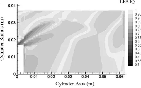
In this research, the LES-IQ has been determined in 75° After Top Dead Center (ATDC) on mentioned grid because in this

crank angle the intensity of turbulence energy is so high. Fig.

3 shows the contour of this index in the above-mentioned

crank angle. This contour illustrates that the value of this

index in most of the computational domain is more than 0.8,

which means that more than 80% of turbulent kinetic energy

is resolved.

In addition to checking the grid resolution with LES-IQ in Fig. 3, Fig. 4 shows the sensitivity of the axial mean velocity to variations in the mesh size. This figure shows the profile

of axial mean velocity at 36° ATDC in the suction stroke.

The location is 20 mm below the cylinder head. To draw this figure, a domain with 5000, 10000 and 20000 computational cell is used. The velocity curve with 10000 cell is so close to

velocity curve with 20000 cell. Thus, with regard to this issue and LES-IQ contour, a computational grid with 20000 cells is

selected in this simulation.

4- 2- Computational time step

The step of crank angle degree has a significant effect on the

precision of computation. Fig. 5 shows the profile of axial

mean velocity per mean piston velocity at 36° ATDC in

suction stroke with different values of crank angle step. The

location is 20 mm below the cylinder head. The mentioned

curve has been drawn for five crank angle steps of 1, 0.5,

0.25, 0.125 and 0.0625. As can be seen in this figure, as the

steps of crank angle become smaller, the velocity profile for

consecutive steps gets closer together. As can be observed, the

velocity profile for steps 0.125 and 0.0625 almost coincide

with each other. Therefore, 0.125 is selected as the final step

of crank angle in this research.

5- Initial and Boundary Conditions

The existing initial condition of air inside the cylinder has

been taken as 300 K and 1 atm and the initial condition of

Fig. 2. Computational grid piston-cylinder assembly with axial symmetry

Cylinder Wall

Moving Boundary

Piston

Valve

Symmetry axis of cylinder

Fig. 3. Contour of LES_IQ in 75 degree crank angle ATDC

Fig. 4. Evaluation of the effect of grid resolution on radial profile of axial mean velocity at 36° ATDC, 20 mm from

cylinder’s head

Fig. 5. Evaluation of the effect of computational time step on radial profile of axial mean velocity at 36° ATDC, 20 mm from

the flow is assumed to be with zero velocity in the whole computational domain. The no-slip condition is applied to the cylinder walls. The temperature of all the walls has been

considered constant and equal to 320 K. Fig. 6 shows the

initial and boundary conditions on the whole computational

domain.

The boundary condition on the symmetry axis of the cylinder

for the whole variables except radial velocity is taken as (∂Φ/∂r)=0.

During engine operation, the inlet velocity of flow into the cylinder is unknown. For the inlet valve equation, it is assumed that the temperature, pressure, and density of fluid into the manifold are specified. When the equation of valve mass flow rate is solved, the inlet velocity for a certain amount of valve opening will be calculated. This velocity has

been considered as the time dependent boundary condition in each crank angle.

For areas close to the walls, standard wall function has been

used. The relation between local shear stress and velocity in

the grid next to the wall is presented as:

µ

ρ

τ = 1/4 1/2₊ p

w

C k u

u (18)

where u+ _{for viscous sublayer and inertial sublayer are defined}

with the following equations [12]:

+₌ +

u y (19)

+₌1 ( )+

u Ln Ey

k (20)

By using wall function, it is not necessary to use very fine

grid near the walls and it can decrease the computational cost.

6- Results and Discussion

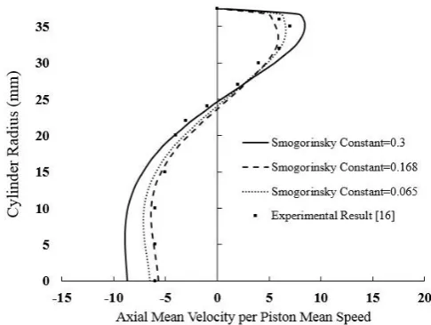
6- 1- Effect of Smogorinsky constant

In the first part of this section, the effect of Smogorinsky

constant on the LES results has been investigated. This

constant is used in the equation for Smogorinsky turbulence

viscosity. Fig. 7 shows the sensitivity of the axial mean

velocity to a Smogorinsky constant at 144° ATDC in the

suction stroke. The location is 20 mm below the head. Similar profiles in different crank angles and also in different

distances from cylinder head are evaluated and at the end, the

best fit with experimental results is obtained with the amount

of 0.168.

6- 2- Verification

The simulation of in-cylinder flow on Imperial College’s

laboratory axisymmetric engine during four consecutive

cycles of suction and compression is performed using the LES turbulence model. To evaluate the effect of initial condition on the flow filed Fig. 8 shows the axial velocity variations in a fixed point of domain near the head of the cylinder during 4

consecutive cycles. As can be observed, after the first cycle,

the variation in axial velocity is repeated frequently. Thus, the

first cycle has not been included in the calculations.

The laboratory results to verify this research are obtained by Morse [16] using laser Doppler anemometry on this engine.

Measured velocity within the cylinder is reported by the radial profile of axial mean velocity and axial root mean

square velocity.

Fig. 9 compares the radial profiles of axial mean velocity in

36 degrees ATDC at the distance 10 mm from the cylinder

head with the experimentalresults and the results from the

standard k-ε model obtained by Liu [10].

Also in Fig. 10, this profile in 144 degree ATDC at the distance

20 mm from the cylinder head, and in Fig. 11 this profile in

90 degree BTDC at the distance 30 mm from cylinder head

are shown.

As seen in Figs. 9, 10 and 11, LES method in the calculation

of mean velocity predicts results that are more accurate, particularly during the suction stroke compared with k-ε

model. This accuracy is more evident in suction stroke rather Fig. 6. Initial and boundary condition on computational

domain Fig. 7. Evaluation of the effect of Smogorinsky constant on

radial profile of axial mean velocity at 144° ATDC, 20mm from cylinder’s head

than compression stroke because in the suction stage the

turbulence intensity is high with regard to the inlet jet flow. Also as seen in Fig. 9, the k-ε model is unable to capture the maximum of mean velocity and its radial location. On the other hand, the weakness of k-ε model is more noticeable when velocity profile is examined in the region near the wall.

By evaluating the whole results obtained from LES and k-ε

models, it can be found that in suction stroke, the differences

between these two models are more significant than

compression stroke and it can be concluded that k-ε model

presents weaker and unreliable results during suction stroke.

However, it should be noted that the LES model is in a good agreement with experimental data in all the crank angles in

the area near the symmetry axis of the cylinder. It is because

of the nature of LES method, which directly solves the large

scale eddies in this area.

Similar profiles for axial mean velocity in 36°, 90°, 144°, and

270° of crank angle and at the distance of 10, 20, 30, 40 and

50 mm from cylinder’s head are obtained in reference [13]. As an average, the mean error of LES method in comparison with experimental data has been obtained to be 26%, while this error in k-ε model is 48%.

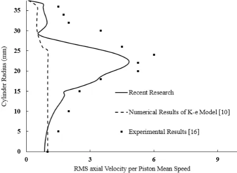
Root Mean Square (RMS) axial velocity profile indicates the level of velocity fluctuation. As the level of velocity fluctuation increases, the turbulence kinetic energy will be increased. In Fig. 12, the radial profiles of axial RMS velocity

in 36 degrees ATDC at the distance of 20 mm from the

cylinder head are shown in comparison with experimental data and Liu numerical results [10].

Also in Fig. 13, the same profile in 144 degree ATDC at the

distance 20 mm from cylinder head is shown. In fact, these

figures show the strength of LES method in calculating the

axial velocity fluctuations. According to Figs. 12 and 13, both levels of fluctuations and their patterns are in very good agreement with the experimental results while k-ε model is

unable to capture these features of the flow characteristics.

Similar profiles for RMS axial velocity in 36°, 90°, 144° and

270° of crank angle and at the distance of 10, 20, 30, 40 and

50 mm from cylinder head are obtained by Khorramdel et al. [13].

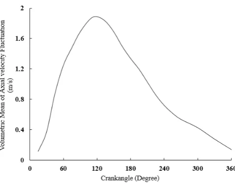
6- 3- Turbulence behavior of flow inside the cylinder

Fig. 14 shows the volumetric mean variation of the axial

velocity fluctuation during suction and compression strokes.

The results show that the axial velocity fluctuations during

suction reach a higher level than in the compression stroke

because of the inlet jet flow to the cylinder and intensive gradient of the flow variables.

Fig. 9. Radial profile of axial mean velocity at 36° ATDC, 10 mm from cylinder’s head

Fig. 10. Radial profile of axial mean velocity at 144° ATDC, 20 mm from cylinder’s head

Fig. 11. Radial profile of axial mean velocity at 90° BTDC, 30 mm from cylinder’s head

With regard to variation of axial velocity fluctuation in Fig.

14, the flow in 100 degree ATDC during intake stroke reaches

the maximum level of turbulence intensity and then the turbulence generated during the intake stroke decays rapidly;

that is, there is hardly any turbulence effect detected during

most of the compression stroke. It seems that the turbulence,

which effects on the combustion process, will be regenerated

in the compression stroke. Similar results are obtained by

Banaiezadeh and colleagues about this phenomenon [17].

During intake stroke when the piston moves from its initial

position at TDC, the air flow enters the cylinder and creates a

jet stream. Along this stroke because of the strong jet stream

and due to the fact that the piston speed will be maximum in

mid-stage, the fluid velocity increases and then by reducing

piston speed, the fluid velocity decreases. Fig. 15 shows the

volumetric mean variation of the fluid velocity during one

cycle.

Fig. 16 shows the stream line of the flow in the beginning of

the suction stroke at 36 degree ATDC. While the accelerated

flow enters the cylinder, one part of it goes straight towards

piston and the other part goes back to the cylinder head and

creates a large scale eddy behind the inlet valve. Also, a smaller circulation area is created at the corner of the cylinder above the inlet valve that rotates in the opposite direction to the large scale eddy behind the inlet valve.

As can be seen in Fig. 17, during the suction stroke, three

main eddies are generated inside the cylinder that will be grown up with increasing the crank angle. At 65 degree

ATDC, a large scale eddy is created near the piston because

of the inlet jet impact to the cylinder wall and moves toward the symmetry axis of the cylinder where a circulation area is

created near the piston. From this crank angle onwards, the

main eddy created behind the inlet valve will be grown up and its center moves toward the cylinder wall.

Fig. 18 shows the stream line of the flow at the end of the

intake stroke. At this time and while the piston reaches

the BDC, suddenly the piston speed becomes zero and the

direction of its movement is reversed. Thus, the flow field

Fig. 13. Radial profile of RMS velocity at 144° ATDC, 20 mm from cylinder’s head

Fig. 14. Volumetric mean variation of the axial velocity fluctuation during one cycle

Fig. 16. Flow Streamlines, inside the cylinder at 36 degree ATDC

becomes unstable and a small eddy is created near the inlet

valve.

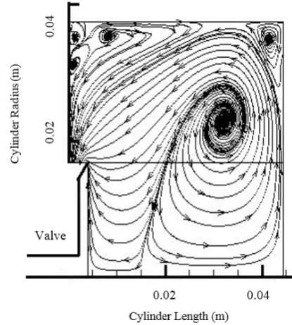
Fig. 19 shows the stream lines of the flow at 90 degree

BTDC within the compression stroke. At this crank angle,

the direction of rotation of eddies is opposite to the one in the suction stroke. The reason for this change is that in

a suction stroke, the inlet fluid velocity and computational

grid movement velocity are in the same direction and they

reinforce each other, while in compression stroke the velocity

of computational grid is in opposite direction of the previous

stage.

In addition to the main eddy inside the cylinder, some smaller

eddies are captured near the cylinder wall because in this area the gradient of fluid velocity is very high. These eddies indicate a good performance of LES method near the walls. In a simulation with k-ε and ASM model, these eddies are not

captured as reported in reference [2].

Fig. 20 shows the stream line of the flow at 30 degree

BTDC. At the end of the compression stroke when the piston

approaches TDC, the coherent structure will not be seen in

the cylinder. At this time, some small circulating area will appear beside the main vortex. In fact, this type of the flow

field at the end ofcompression stroke assists fuel-air mixing

while fuel is injected into the cylinder.

7- Conclusions

In this research, a study on the simulation of in-cylinder

flow in internal combustion engine using LES method with

Smogorinsky submodel is done. This model is applied to the

axisymmetric engine with the flat cylinder head, a piston and

a fixed valve.

According to the results, the LES method is more accurate in calculating the mean velocity values compared with k-ε

model especially over the intake stroke where the level of turbulence is so high due to inlet jet flow. The observed mean velocity profiles in areas near the walls during the

intake stroke demonstrated the weaknesses of k-ε model. By

evaluating whole results obtained from LES and k-ε model, it

was found that during suction stroke the differences between

these two models are greater than those over the compression

stroke, which can be said that k-ε model presents weak and

unreliable results in compression stroke. However, it should be noted that the LES model in all aspects near the axis of

Fig. 17. Flow Stream lines, inside the cylinder at 65 degree ATDC

Fig. 18. Flow Stream lines, inside the cylinder at BTDC

Fig. 19. Flow Stream lines, inside the cylinder at 90 degree BTDC

symmetry has shown better results than the k-ε model, compared with experimental data. This is because of the nature of LES model, which directly solves the large scale eddies of the flow in this area.

With regard to RMS velocity profiles in this research, it was observed that the level of fluctuations and its pattern are in very good agreement with the experimental results while k-ε model is unable to capture this feature of the flow.

Another issue that is investigated in this research is the effect

of Smogorinsky constant value on LES results. This constant

has a major effect on mean and RMS velocity profiles. In

this simulation by evaluating the results, the best fit with

experimental data was achieved with the amount of 0.168.

Nomenclature

Smogorinsky Constant

C_s

Cross Stress, Kg.m-1_s-2

C_i,j

Filter Function

G

Enthalpy, m2_.s-2

h

Kinetic Energy, m2_.s-2

k

Leonard Stress, kg.m-1_s-2

L_i,j

Pressure, kg.m-1_s-2

P

Prandtl Number Pr

Reynolds Stress, kg.m-1_s-2

R_i,j

Cylinder Radius, m r

Strain Rate Tensor, s-1

S

Temperature, K

T

Time, s

t

Velocity, m.s-1

u

Grid scale Velocity, m.s-1

<u>

Sugrid Scale Velocity, m.s-1

u΄

Local Reynolds Number

y+

Turbulence Kinetic Energy Constant

C_I

Greek Symbols

Density, kg.m-3 ρ

Dynamic Viscosity, kg.m-1_s-1

μ

Kinematic Viscosity, m2_s-1

v

Smogorinsky Kinematic Viscosity, m2_s-1

v_sgs

Filter Width, m

Δ

Subgrid Stress Tensor, kg·m-1_s-2

τ_sgs

Superscript and subscript Subgrid Scale SGS

Grid Scale GS

References

[1] N. Mosleh, H.Khaleghi, Simulation of flow into the internal combustion engine using K-ε, MSc thesis,

Tarbiat Modares University, Tehran, (1997).

[2] M. Fallah, Khaleghi, H, Calculations of flows in

reciprocating engine chambers with AMS & K- ε, 1st

International conference of computational methods in

applied mathematics, Belarus, (2003).

[3] K. Naitoh, K. Kuwahara, Large eddy simulation and direct

simulation of compressible turbulence and combusting

flows in engines based on the BI-SCALES method, Fluid Dynamics Research, 10(4-6) (1992) 299-325.

[4] F. Bottone, A. Kronenburg, D. Gosman, A. Marquis, Large eddy simulation of diesel engine in-cylinder flow,

Flow, turbulence and combustion, 88(1) (2012) 233-253.

[5] V. Huijnen, L. Somers, R. Baert, L. de Goey, C. Olbricht,

A. Sadiki, J. Janicka, Study of turbulent flow structures

of a practical steady engine head flow using large-eddy

simulations, Journal of Fluids Engineering, 128(6) (2006) 1181-1191.

[6] R. Verzicco, J. Mohd-Yusof, P. Orlandi, D. Haworth, LES in complex geometries using boundary body forces, Center for Turbulence Research Proceedings of the

Summer Program, NASA, Stanford University, (1998)

171-186.

[7] I. Celik, I. Yavuz, A. Smirnov, Large eddy simulations of

in-cylinder turbulence for internal combustion engines: a

review, International Journal of Engine Research, 2(2)

(2001) 119-148.

[8] D. Haworth, Large-eddy simulation of in-cylinder flows, Oil & Gas Science and Technology, 54(2) (1999) 175-185.

[9] I. Celik, I. Yavuz, A. Smirnov, J. Smith, E. Amin, A. Gel, Prediction of in-cylinder turbulence for IC engines, Combustion science and technology, 153(1) (2000) 339-368.

[10] K. Liu, Large-eddy simulation of in-cylinder flows

in motored reciprocating-piston internal combustion

engines, The Pennsylvania State University, 2012.

[11] L. Davidson, Fluid mechanics, turbulent flow and

turbulence modeling, Chalmers University of Technology,

(2012).

[12] A. Yoshizawa, Statistical theory for compressible

turbulent shear flows, with the application to subgrid

modeling, The Physics of fluids, 29(7) (1986) 2152-2164.

[13] M. Khorramdel, Khaleghi, H, Investigation of

in-cylinder flow in internal combustion engines by LES method, MSc thesis, Tarbiat Modares University, Tehran., (2014).

[14] M. Klein, An attempt to assess the quality of large eddy

simulations in the context of implicit filtering, Flow, Turbulence and Combustion, 75(1) (2005) 131-147. [15] M. Klein, J. Meyers, B.J. Geurts, Assessment of LES

quality measures using the error landscape approach,

in: Quality and Reliability of Large-Eddy Simulations, Springer, 2008, pp. 131-142.

[16] A.P. Morse, Turbulent flow measurement by

laser-doppler anemometry in motored piston-cylinder

assemblies, Transactions of the ASME., , Vol 101, (pp. 208–216.) (1979).

[17] A. Banaeizadeh, A. Afshari, H. Schock, F. Jaberi,

_

_ ~

Large-eddy simulations of turbulent flows in internal

combustion engines, International Journal of Heat and

Mass Transfer, 60 (2013) 781-796.

Pleasecitethisarticleusing:

M. Khorramdel, H. Khaleghi, Gh. Heidarinejad, M. H. Saberi, “Numerical Analysis of In-Cylinder Flow in Internal Combustion Engines by LES Method”, AUT J. Mech. Eng., 1(1) (2017) 29-38.