AUT J. Mech. Eng.,4(2) (2020) 241-256 DOI: 10.22060/ajme.2019.15690.5790
A Changing-Connectivity Moving Grid Method for Large Displacement
M. M. Razzaghi*
Department of Mechanical Engineering, Najafabad Branch, Islamic Azad University, Najafabad, Iran
ABSTRACT: A moving grid method is introduced in this paper and different motions of the body
are simulated using this method. This study indicates that by regular and systematic change of grid connections in some elements with regard to the size of the body’s motion, a moving-grid can be obtained which is capable of being adapted to the large motions of the body without reducing the quality of elements. In order to model the rotational or translational motions of the body, cylindrical or elliptical shells from the elements around the body are taken into consideration to change the grid connections. To indicate the correct performance of introduced moving-grid method, several test cases including rotational and translational motions are solved. The Euler equations in the three dimensional unsteady form is solved using a dual time implicit approach. Numerical dissipative term using Jameson method is added to the equations. To accelerate convergence, local pseudo-time stepping, enthalpy damping and residual averaging are used. The results are validated with experimental or numerical data and excellent agreements among the results are observed.
Review History: Received: 23 Jan. 2019 Revised: 17 Jul. 2019 Accepted: 31 Jul. 2019 Available Online: 15 Sep. 2019
Keywords: Moving-grid Grid connections Translational motion Unsteady 1- Introduction
A variety of time dependent applications can be found in literature. These include flutter analysis, store separation, analysis of flow around helicopter blades in forward flight and rotor-stator combination in turbomachinery. Most of these applications are concerned with the complex geometries with moving boundaries. For evaluation of flow field properties in these applications, it is necessary to develop improved solvers and moving grid methodologies.
For a moving boundary problem, the computational grid must move with the moving boundaries. The primary method in this regard is to regenerate the grid around the body after each step of its motion. Despite its simplicity, this method is not efficient since grid regeneration for complex geometries is too difficult. Being time-consuming and requiring a great deal of data interpolation are among other disadvantages of this method [1,2].
The sliding mesh techniques were introduced for the first time by Rai [3,4]. In this technique, two different parts of the grid can slide on each other. Sliding mesh technique is mostly used in Turbomachinery in which one of the grids is related to the stator (fixed) and the other is related to the rotor (moving). Two methods can be used in this technique; the first one is based on the topological changes technology. The second one is the General Grid Interface (GGI).
The first method can be time-consuming, as it needs to re-organize the topology and the internal numbering of
faces and cells at each time step. In GGI method, weighted interpolation is used to evaluate and transmit flow values. The GGI weighting factors are basically the percentage of surface intersection between two overlapping faces. This method needs a specific algorithm which results in many issues in the process of simulation [5-7].
In the dynamic grid, displacements and changes of the body are transferred to grid elements. One of these methods is simulation of nodes connection with springs. In this technique, it is supposed that the nodes are connected by springs. After each change in the situation of the body, a process of making the grid uniform is conducted by balancing the force of the springs [8]. Spring factor can be the same in the whole domain [9] or different in various zones. The reason is decreasing deformations in the zones that nodes are closer to each other [10,11]. In some of the research works, torsion springs are used in order to prevent the interference of elements [12,13]. Generally, using this technique in large displacements can reduce grid quality and, in some cases, grid regeneration is needed locally.
the grid is felt.
The overset grid method is introduced for cases where large displacements of the body occur. The most famous method in this category is the chimera grid. Chimera grid is made up of two grids: the main grid and the local grid. The local grid, along with the body, moves on the main grid. Transfer of information between local and main grids is difficult. Therefore, it usually requires a structured grid or at least a Cartesian unstructured grid. But recently, unstructured grids are also used in the chimera grid method. Repeated interpolations in this method reduce the accuracy of solution [18-23].
Most of the current methods endeavor to fix grid connections as much as possible. Reduction of the grid quality and limitation of body movements are among the drawbacks of these methods. Additional details and some of the applications of the mentioned methods are presented in references [24-28].
In the present study, the flexibility of grid has been increased regarding the idea of change in the grid connections. To this end, some of the grid elements have been considered as a deformable shell. This shell is modified simultaneously by the rotation or translation of the body. In the moving-grid defined here, in addition to the ability of modeling the large movements of the body, the primary quality of elements is retained and there is no need for transferring data between different parts of the grid, regenerating the grid, deletion/insertion of nodes, and repeated interpolations. As for a limitation of the defined moving grid method, the incapability of modeling the simultaneous motions of two bodies with a small distance can be mentioned.
To validate and demonstrate the correct performance of the 3 Dimensional (3D) moving-grid, several test cases including rotational and translational motions have been considered. Therefore, the 3D unsteady form of the Euler equations is solved. An averaging method is used for calculating the properties over each cell faces. Also, numerical dissipative term using Jameson method is added to the equations [29,30]. An implicit dual time method is
used for time integration of equations [31-33].
The obtained results of several test cases are compared with experimental or other numerical data.
2- Grid Configuration
Most of the current methods keep the mesh connections stable in order to prevent configuration of the mesh from disruption. But it reduces the quality of the mesh and limits the movements of the body in the domain.
With the change in the mesh connections, a flexible mesh with high performance can be obtained. But, making change in the mesh connections without any clear planning and order may lead to disruption and disorganization in the mesh. Therefore, any change in the connections must be made only in a limited number of the elements. The manner of arrangement and the place of these elements are so vital for having a clear order and obtaining a regular method.
The elements which are considered as for changing the connections must form a closed ring so that the idea of changing connections in a regular and permanent manner will be applicable. The place of this closed ring must be chosen with regard to the type of the body’s motions. Any kind of the body’s movement can be divided into rotational and translational motions.
2- 1- Rotational motions
In order to model the rotational motions of the body, a cylindrical shell from the elements which are around the body will be taken into consideration to change the connections. Thus, the mesh is divided into 2 zones: the first zone consists of the elements which are placed between the body and the cylindrical shell. The second zone includes the elements outside the ring to the outer boundaries of the domain.
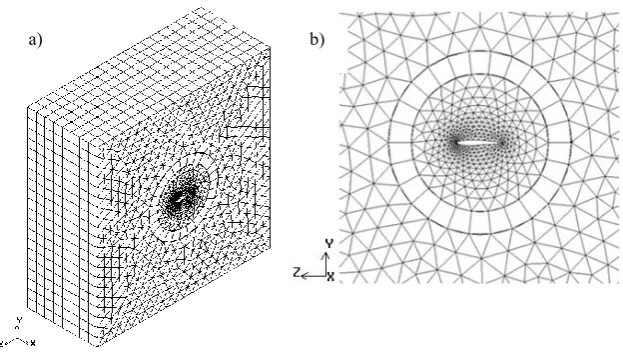
In Fig. 1, the cylindrical shell around a rectangular wing for a three-dimensional domain with outer cubical boundaries is shown. In Fig. 2, the domain is shown completely along with the elements in the first and second zones.
In order to model the rotational motions of the body, there is a need for the elements of the first zone to rotate along with the body while the elements of the second zone have to be
Fig. 1. Cylindrical shell around a rotational body (oscillatory wing); a) 3D view; b) 2D view
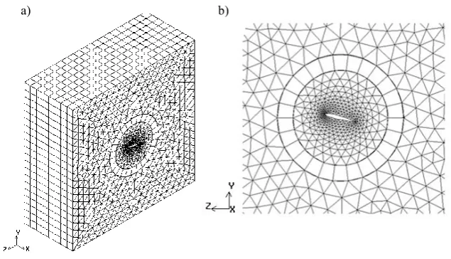
totally motionless. Therefore, the elements within the shell get deformed (See Fig. 3).
This way, other elements of the mesh which are outside the shell will not become deformed. As a result, firstly, the quality of other elements which include most of the mesh’s elements is retained. Secondly, the quality of the elements that are close to the body’s surface is maintained. These elements are of high importance due to being small and the occurrence of flowing phenomena in them. Thirdly, with the distinction of the deformed elements there isn’t any need to control the quality of all the elements or search to find the defective elements and finally, geometrically desirable elements with more
lasting quality and higher deformation tolerance can be used in this shell.
However, the capacity of these elements’ tolerance for deformations is limited and therefore, it may cause problem in the large rotations of the body. To offer a solution for this problem, the idea of change in the mesh’s connections can be used. Consequently, with every node reaching its neighbor node in the cylindrical shell, the mesh’s connections get modified (See Fig. 4).
If it is supposed that there are n nodes on each of the borders around the cylindrical shell, after the 360/n degree rotation of the body every node on the interior border of the shell with the first zone will reach the
Fig. 3. The mesh after the wing rotation along with the elements between wing and
cylindrical shell (zone 1); a) Complete view of domain; b) Close up view b)
a)
Fig. 2. Unstructured grid along with cylindrical shell around the wing (before rotation); a) Complete view of domain; b) Close up view
position of its neighbor node prior to the rotation. In this position, the previous connections are replaced with the new connections in a way that each node connects with the node facing it in the new position. Hence, the deformations are controlled and the quality of elements returns to its primary state. The process of changing connections on one of the rings of the cylindrical shell after the 360/n degree rotation of the body is shown in Fig. 5.
Considering the size of the body’s rotation and the repetition of this process, the high-degree rotation of the body can be modeled without any concern for reduction of the elements’ quality and disruption of the mesh’s configuration (See Fig. 6).
It is worth mentioning that any geometric shape can be used for the elements of the cylindrical shell. However, regarding the existing geometrical symmetry in the hexahedral elements which enhance the ability to bear these deformations in this type of the element, this geometric shape was used for the elements of the
cylindrical shell. Of course, the process of changing connections for this type of the element is applicable much more easily. In equal conditions, with regard to the number of nodes and the dimensions of the cylindrical shell, employing hexahedral elements in the mesh lead to the reduction of the number of elements in this shell. The comparison between the number of required elements for building the cylindrical shell using the hexahedral elements and the wedge is illustrated in Fig. 7. As it is demonstrated in the above-mentioned figure, the number of required elements for the elements of the wedge is twice as the number of hexahedral elements. It is evident that this number will increase using the pyramidal or tetrahedral elements.
In order to have more symmetrical elements and making the form of the hexahedral elements of cylindrical shell close to a cubical form, it is necessary to select the number of elements with regard to the thickness of the cylindrical shell. Thus, as the thickness of the cylindrical shell decreases the number of the nodes and
Fig. 4. The mesh after the wing rotation along with the elements of zone1 and changes in connections of the cylindrical shell; a) Complete view of domain; b) Close up view
A2 A3 A4 A5 A6 A1 An An-1 An-1 An
A1 A2 A3 A4 A5
A6
A1 A2 A3 A4 A5 An An-1 An-2 An-1 An
A1 A2 A3 A4 A5
A6 a)
c)
A1 A2 A3 A4 A5 An An-1 An-2 An-1 An
A1 A2 A3 A4 A5
A6
A1 A2 A3 A4 A5 An An-1 An-2 An-1 An
A1 A2 A3 A4 A5
A6 b)
d)
Fig. 5. Connections change process in the cylindrical shell (a) Before rotation; (b) After rotation of zone 1; (c) After rotation when each node on the inner part reaches the previous position of its
neighbor node; (d) After rotation and change in nodes connection
a) b)
Fig. 6. The grid after 70° rotation of the wing and 5 step changes in connections of the cylindrical shell; a) Complete view of domain; b) Close up view
a) b)
Fig. 7. The comparison of two geometric forms of elements for the cylindrical shell; a) Hexahedral form (286 elements); b) Wedge form (572 elements)
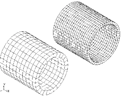
the elements on the shell have to be increased (See Fig. 8). To prevent disorder in changing the connections, it is better to utilize a layer of elements for making the cylindrical shell (See Fig. 9).
The type of the element which has been used for the mesh of the zone 1 and 2 doesn’t affect the configuration of the mesh and can be selected with regard to the existing limitations of the problem at hand. Considering the advantages of the unstructured method in the mesh generation around the complex geometries and the more distinctive features of the deformable shell in Figs. 2 to 4, pyramidal and tetrahedral elements have been used in zone 1 and 2. Pyramidal elements have been applied only in the vicinity of the cylindrical shell and the rest of the zone 1 and 2 is covered with tetrahedral elements.
But in general, this method has been devised for the rotation of a body around an axis. If the simultaneous rotation of the body around several axes is considered, a sphere has to be used instead of a cylinder.
2- 2- Translational motions
As for modeling the translational motions of the body, two shells with elliptical sections should be employed. The manner of placing these shells is shown in Fig. 10. Accordingly, the mesh in the solution Domain is divided into three zones. The first zone includes the elements in
the inner shell. The second zone consists of the elements between the two shells and the body. The third zone contains the elements between the outer shell and the outer boundaries of the domain (See Fig. 11).
Simultaneous with the movement of the body, the elements of the second zone move along with the body and the elements of the first and the third zone remain stable. This way, the elements within the two shells are deformed. In this situation, with the regular changing of the connections, the translational motions of the body can be modeled without causing disruption in the configuration of the mesh. The modeling of the translational motion using the rotating shells is very much similar to the translation of the body on a specific path on the conveyer which is used in the mines and factories. The length of the shells is adjustable according to the range of the translational motion which has been considered for the body. Also, the distance between the two shells is determined by taking the size and dimensions of the body
Fig. 10. Two shells around a translational body (wing) in 3D view
Fig. 11. Two shells around a translational body (wing) in 2D view
a) b)
Fig. 12. The unstructured mesh along with the shells around translational wing (before translational motion)
Fig. 13. The mesh after translational motion of the wing along with the elements of zone 2
into consideration.
Just like the rotational movements, there isn’t any limitation regarding the form of the elements. Therefore, regarding the previously mentioned advantages of the hexahedral elements, these types of the elements have been used in the shells. The tetrahedral and pyramidal elements are used for the rest of the mesh in the domain. The translational motion of an airfoil, the deformations in the two shells as well as the changing of these elements’ connections is illustrated two-dimensionally in Figs. 12 to 14.
4- 1- Rotational and translational motions
In order to model the rotational and translational motions of the body simultaneously, both of the previous positions
must be combined together. In other words, a cylindrical shell around the body and two other shells in the direction of the translational motions must be used (See Fig. 15). All the points mentioned for the two previous states are also the same for this state and therefore, will not be repeated again.
It is worth mentioning that by changing the form and dimensions of the shells and using the idea of making change in the connections, any kind of the body’s motion can be modeled.
5- Solution Algorithm
0
Q
F
G
H
t
x
y
z
+
+
+
=
(1) (1)where Q is the vector of state variables and F, G and H denote the convective fluxes in the corresponding x, y and z coordinate directions.
The Eq. (1) are augmented by the equation of state, which for a perfect gas is given by
(
1
)
2 2 22
u v
w
P
=
γ
−
ρE ρ
−
+
+
(2)(2)where P is the pressure, ρ is the density, γ is the ratio of specific heat,
(
u v w, ,)
are the three Cartesian velocity components, and E is the total energy of the flow.For a control volume with volume V and surface S, Eq. (1) can be rewritten in integral form as
Fig. 15. Three shells around a moving body (translational and rotational wing) Fig. 14. The mesh after the wing translation along with the elements of zone2 and changes in
v s
(
F
G
H
)
0.
QdV
dS
t
x
y
z
+
+
+
=
(3) (3)Appling Eq. (3) to each cell in the domain independently, the spatial and time dependent terms are decoupled and a set of Ordinary Differential Equation`s (ODE) is obtained in the following form
(
i i)
i( )
0
d QV R Q
dt
+
=
(4)(4)That first term of above equation indicant change in control-volume depend of time and R Qi
( )
is the convective fluxes of cell faces. Where Vi is the cell volume, considering the fact that in rotational displacements the form of the elements outside the shell is constant, these elements will have no volume change in relation to time. Of course, no volume changes occur in the shell in rotational displacements due to the existence of symmetry (see Fig. 16).Therefore, it can be concluded that the volume of all elements is constant in relation to time and Eq. (6) can be rewritten accordingly for rotational displacements:
Fig. 16. Comparison of the elements volume in the cylindrical shell (2D view); a) Before rotation; b) After rotation
Table 1. Turbine characteristics
Description Test 1 Test 2 Test 3
Mach number 0.5 0.85 1.2
Angle of attack 0 1 7
Chord length 1 1 1
Wing span 4 4 4
( )
( )
0
i i i
d
V
Q
R Q
dt
+
=
(5)(5)whereVi is the cell volume of each element, dtd Q( )i indicant change in control-volume depend of time and R Qi
( )
isthe convective fluxes of cell faces.
With regard to the fact that the elements’ surface changes in the state of translational motions, in general, Eq. (4) is considered.
The properties over each cell faces are evaluated using an averaging method. In this method added numerical dissipative term to Eq. (4) with using Jameson method.
(
i i)
i( )
i( )
0
d QV R Q D Q
dt
+
−
=
(6)(6)A dual time stepping scheme was used to solve the equations at each time step.
3- Numerical Result
The experimental and numerical results are compared and presented in this part. A rectangular wing with NACA0012 airfoil is considered.
In the first phase, the flow was simulated around a motionless wing. The conditions of flow are demonstrated in Table 1.
Specifications of the three used meshes for the grid study are shown in Table 2.
In Figs. 17 to 19, obtained results are compared with
Table 2. Mesh specifications
Mesh type Number of nodes number of
elements Number of nodeson the airfoil Number of faceson the outer boundary
Coarse 52255 82760 100 41492
Middle 119550 190232 150 95228
Fig. 17. The NACA0012 airfoil in subsonic flow with M∞=0.5,∝=0° ; a) Comparison of the pressure
distribution; b) The pressure and velocity contours
Fig. 18. The NACA0012 airfoil in transonic flow with M∞=0.85,∝=1°; a) Comparison of the pressure
Fig. 19. The NACA0012 airfoil in supersonic flow with M∞=1.2,∝=7°; a) Comparison of the pressure
distribution; b) The pressure and velocity contours
Description
Test 1
Test 2
AGARD number
CT1
CT5
Mean angle of attack (
𝛼𝛼
𝑚𝑚)
2.89
0.016
Angle of attack variation (
𝛼𝛼
0)
2.41
2.51
Mach number
0.6
0.755
Reduced frequency (
K
c)
0.0808
0.0814
Table 3. AGARD test case descriptions
AGRAD-211 data. The results indicate that the grid performed very well.
In the second phase, the oscillatory wing was studied. The characteristics of the tests are summarized in Table 3. Results shown in Fig. 20 confirm the accuracy and efficiency of this method.
The comparison of grids specifications and computational timings obtained from the presented method and two other moving grid methods are demonstrated in Table 4 [34]. It is seen that the number of elements as well as the computational timing reduces in this method which is a very valuable feature. This is due to eliminating the total and local mesh regeneration, obviating the need for usual interpolations in moving grids, obviating the need to use several series of local and background grids and transferring information between them, and obviating the need to calculate the surface of elements in every time step.
In the third phase, the unsteady flow around a wing with NACA 0012 airfoil moving with the speed of Mach 0.5 in stationary air was simulated. After the initial translation, the flow domain around the moving wing should become steady with respect to the wing. Pressure contours on the wing surface at the middle of span after six chord translations are presented in Fig. 21(a).
The CP distributions along the wing surface at the middle of span from steady state and translational wing are compared with each other in Fig. 21(b). It is seen that the agreement is excellent.
Fig. 20. Comparison of normal force coefficient from computational with a) CT1 test case; b) CT5 test case
a) b)
Fig. 21. a) Pressure contours after six chord translations; b) Comparison of pressure distribution from stationary wing with moving flow and stationary air with moving wing
Grid type Number of elements
Time
divided by iterations and number of elements
Overset 212937 4.649 × 10⁻⁴
Spring 97245 5.562 × 10⁻⁴
Present 6030 1.100 × 10⁻⁵
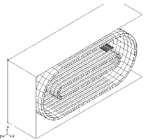
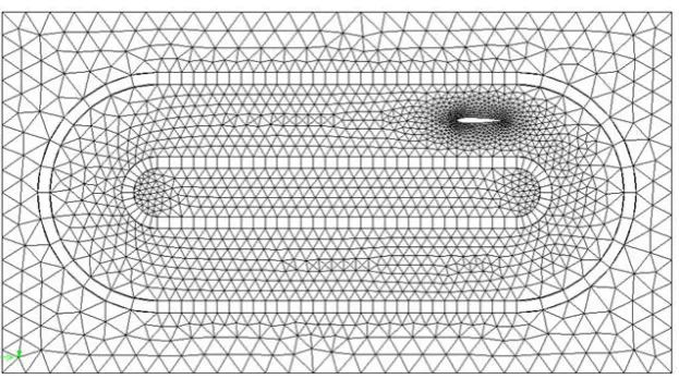
Fig. 22. Computational model and mesh configuration, a) Complete view of domain, b) Close up view
elements are smaller. Therefore, in the presented method, fewer computations are needed and also the computational timing takes a shorter period of time.
In the 4th phase, the effect of rotor blades movement on stator’s blade was investigated in turbomachinery. The findings of this study were compared with those of reference [35].Cross section of rotor blades is NACA0024 with a chord length of 50 mm. The blade spacing of rotor is 0.1 m. A stator blade in a real machine is represented by the flat plate where its elliptic leading edge is located 40 mm downstream from the trailing edge of the airfoils (Fig. 22). The free stream velocity was set to 3.0 m / s for all experiments. The speed of the rotor blades was selected 0, 2, 3 and 4 m / s. Fig. 23 shows the comparison between numerical results and the experimental results for the boundary layer velocities on stator plate. The validation shows a good agreement between the implemented numerical model and experimental results.
4- Conclusion
In this study, cylindrical or elliptical shells from the grid elements around the body are taken into consideration in order to change the grid connections. These shells are modified simultaneously by the rotation or translation of the body.
The results of the study revealed that large displacements of the body can be simulated using the introduced method. Moreover, the idea of regular manipulation of grid connections avoids reduction of the grid quality. Simplicity of the method and shorter Central Processing Unit (CPU) time are among other advantages of this method. Using this method for simulation of different moving bodies is suggested.
References
[1] A. Goswami, I. Parpia. Grid restructuring for moving boundaries, In: 10th Computational Fluid Dynamics Conference, 1991.
[2] A. L. Gaitonde, S. P. Fiddes. A three-dimensional moving
𝐶𝐶𝑝𝑝 pressure coefficient
𝐶𝐶𝑛𝑛 normal force coefficient
𝐶𝐶𝑚𝑚 pitching moment coefficient c chord
E total energy
F convective flux in the x direction
G convective flux in the y direction
H convective flux in the z direction
K reduce frequency
M Mach number
P pressure
Q vector of conserved variable
S surface
t time
u x component of Cartesian velocity
v y component of Cartesian velocity
w z component of Cartesian velocity
𝑢𝑢𝑟𝑟 relative velocity in the x direction
𝑣𝑣𝑟𝑟 relative velocity in the y direction
𝑤𝑤𝑟𝑟 relative velocity in the z direction V volume
𝑥𝑥𝑡𝑡 velocity of control-volume boundary in
the x direction
𝑦𝑦𝑡𝑡 velocity of control-volume boundary in
the y direction
𝑧𝑧𝑡𝑡 velocity of control-volume boundary in
the z direction
α angle of attack
γ ratio of specific heat
𝜌𝜌 density
𝜏𝜏 pseudo-time
𝜔𝜔 angular frequency
NOMENCLATURE
Spring method method Present percentage improving
Number of nodes 3500 2913 20
Number of elements 6850 2789 145.6
Surface of domain 1963.5* 420† 367.5
Size of translation‡ 6 12 100
*Circle with d=50 Chord
† rectangular 28*15 Chord ‡Chord
mesh method for the calculation of unsteady transonic flows, The Aeronautical Journal, 984(1995) 150-160. [3] M. M. Rai, An implicit, conservative, zonal-boundary
scheme for Euler equation calculations, Computers & fluids, 14(1986) 295-319.
[4] M. M. Rai, A conservative treatment of zonal boundaries for Euler equation calculations. Journal of Computational Physics. 62(1986) 472-503.
[5] S. Huang, A. A. Mohamad, K. Nandakumar, Z. Y. Ruan, D. K. Sang. Numerical simulation of unsteady flow in a multistage centrifugal pump using sliding mesh technique, Progress in Computational Fluid Dynamics, An International Journal, 10(2010) 239-245.
[6] M. Beaudoin, H. Jasak. Development of a Generalized Grid Mesh Interface for Turbomachinery simulations with OpenFOAM, In: Open source CFD International conference, 2008.
[7] O. Petit, M. Page, M. Beaudoin, H. Nilsson. The ERCOFTAC centrifugal pump OpenFOAM case-study, In: Proceedings of the 3rd IAHR International Meeting of the Workgroup on Cavitation and Dynamic Problem in Hydraulic Machinery and Systems, Brno, Czech Republic, 2009.
[8] J. T. Batina. Unsteady Euler airfoil solutions using unstructured dynamic meshes, AIAA Paper No. 89-0115, In: AIAA 27th Aerospace Sciences Meeting Kc Exhibit, Reno, 1989.
[9] J. Hase, D. Anderson, I. Parpia. A Delaunay triangulation method and Euler solver for bodies in relative motion, In: 10th Computational Fluid Dynamics Conference, 1991. [10] J. T. Batina. Unsteady Euler algorithm with unstructured
dynamic mesh for complex-aircraft aerodynamic analysis, AIAA journal, 29(1991) 327-333.
[11] S. Pirzadeh. An adaptive unstructured grid method by grid subdivision, local remeshing, and grid movement, In: 14th Computational Fluid Dynamics Conference, 1999.
[12] C. Degand, C. Farhat. A three-dimensional torsional spring analogy method for unstructured dynamic meshes, Computers & structures, 80(2002) 305-316.
[13] D. Zeng, C. R. Ethier. A semi-torsional spring analogy model for updating unstructured meshes in 3D moving domains, Finite Elements in Analysis and Design, 41(2005) 118-139.
[14] L. P. Zhang, Z. J. Wang. A block LU-SGS implicit dual time-stepping algorithm for hybrid dynamic meshes, Computers & fluids, 33(2004) 891-916.
[15] S. M. Mirsajedi, M. S. Karimian, M. Mani. A multizone moving mesh algorithm for simulation of flow around a rigid body with arbitrary motion, Journal of fluids engineering, 128(2006) 297-304.
[16] S. M. Mirsajedi, M. S. Karimian, Evaluation of a two-dimensional moving-mesh method for rigid body motions, Aeronautical Journal, 110(2006) 429-438. [17] S. M. Mirsajedi, M. S. Karimian, Unsteady flow
calculations with a new moving mesh algorithm, In: 44th AIAA Aerospace Sciences Meeting and Exhibit, 2006. [18] S. Zhang, J. Liu, Y. Chen, X. Zhao. Numerical
Simulation of Stage Separation with an Unstructured Chimera Grid Method, In: 22nd Applied Aerodynamics Conference and Exhibit, 2004.
[19] F. Togashi, Y. Ito, K. Nakahashi, S. Obayashi. Extensions
of overset unstructured grids to multiple bodies in contact, Journal of Aircraft, 43(2006) 52-57.
[20] J. Liu, H. U. Akay, A. Ecer, R. U. Payli. Flows around moving bodies using a dynamic unstructured overset-grid method, International Journal of Computational Fluid Dynamics, 24 (2010) 187-200.
[21] R. Kannan, Z. J. Wang. A Parallel Overset Adaptive Cartesian/Prism Grid Method for Moving Boundary Flows, In: Computational Fluid Dynamics, Springer, Berlin, Heidelberg, 2009, pp. 323-328.
[22] R. Kannan, Z. J. Wang. Overset adaptive Cartesian/ prism grid method for stationary and moving-boundary flow problems, AIAA journal, 45(2007) 1774-1779. [23] J. Cai, H. M. Tsai, F. Liu. A parallel viscous flow
solver on multi-block overset grids, Computers & fluids, 35(2006) 290-301.
[24] T. E. Lee, M. J. Baines, S. Langdon. A finite difference moving mesh method based on conservation for moving boundary problems, Journal of Computational and Applied Mathematics, 288(2015) 1-7.
[25] M. M. Razzaghi, S. M. Mirsajedi. A 3-D Moving Mesh Method for Simulation of Flow around a Rotational Body, Journal of Applied Fluid Mechanics, 9(2016) 1023-1034. [26] K. Ou, A. Jameson. Towards computational flapping
wing aerodynamics of realistic configurations using spectral difference method, In: 20th AIAA Computational Fluid Dynamics Conference, 2011.
[27] K. Ou, P. Castonguay, A. Jameson, 3D flapping wing simulation with high order spectral difference method on deformable mesh, In: 49th AIAA Aerospace Sciences Meeting including the New Horizons Forum and Aerospace Exposition, 2011.
[28] M. M. Razzaghi, S. M. Mirsajedi. A moving mesh method with defining deformable layers, Progress in Computational Fluid Dynamics, an International Journal. 17(2017) 63-74.
[29] A. Jameson, W. Schmidt, E. Turkel. Numerical solution of the Euler equations by finite volume methods using Runge Kutta time stepping schemes, In: 14th fluid and plasma dynamics conference, 1981.
[30] A. Jameson, D. Mavriplis. Finite volume solution of the two-dimensional Euler equations on a regular triangular mesh, AIAA journal, 24(1986) 611-618.
[31] A. L. Gaitonde, S. P. Fiddes. A three-dimensional moving mesh method for the calculation of unsteady transonic flows, The Aeronautical Journal, 99(1995) 150-160.
[32] A. Jameson. Time dependent calculations using multigrid, with applications to unsteady flows past airfoils and wings, In: 10th Computational Fluid Dynamics Conference, 1991.
[33] A. Jahangirian, M. Hadidoolabi. An implicit solution of the unsteady navier-stokes equations on unstructured moving grids. In: 24th International Congress of the Aeronautical Science, 2004.
[34] C. Hoke, R. Decker, R. Cummings, D. McDaniel, S. Morton. Comparison of overset grid and grid deformation techniques applied to 2-dimensional NACA airfoils. In: 19th AIAA Computational Fluid Dynamics, 2009. [35] Z. Gete, R. L. Evans, An experimental investigation