https://doi.org/10.5194/gmd-12-4409-2019 © Author(s) 2019. This work is distributed under the Creative Commons Attribution 4.0 License.
Simulating lightning NO production in CMAQv5.2:
performance evaluations
Daiwen Kang1, Kristen M. Foley1, Rohit Mathur1, Shawn J. Roselle1, Kenneth E. Pickering2, and Dale J. Allen2 1Center for Environmental Measurement and Modeling, U.S. Environmental Protection Agency, Research Triangle Park, NC 27711, USA
2Department of Atmospheric and Oceanic Science, University of Maryland, College Park, MD, USA
Correspondence:Daiwen Kang ([email protected]) Received: 11 April 2019 – Discussion started: 29 April 2019
Revised: 3 September 2019 – Accepted: 10 September 2019 – Published: 21 October 2019
Abstract. This study assesses the impact of the lightning nitric oxide (LNO) production schemes in the Community Multiscale Air Quality (CMAQ) model on ground-level air quality as well as aloft atmospheric chemistry through de-tailed evaluation of model predictions of nitrogen oxides (NOx) and ozone (O3) with corresponding observations for the US. For ground-level evaluations, hourly O3 and NOx
values from the U.S. EPA Air Quality System (AQS) mon-itoring network are used to assess the impact of differ-ent LNO schemes on model prediction of these species in time and space. Vertical evaluations are performed using ozonesonde and P-3B aircraft measurements during the De-riving Information on Surface Conditions from Column and Vertically Resolved Observations Relevant to Air Quality (DISCOVER-AQ) campaign conducted in the Baltimore– Washington region during July 2011. The impact on wet deposition of nitrate is assessed using measurements from the National Atmospheric Deposition Program’s National Trends Network (NADP NTN). Compared with the Base model (without LNO), the impact of LNO on surface O3 varies from region to region depending on the Base model conditions. Overall statistics suggest that for regions where surface O3 mixing ratios are already overestimated, the corporation of additional NO from lightning generally in-creased model overestimation of mean daily maximum 8 h (DM8HR) O3by 1–2 ppb. In regions where surface O3is un-derestimated by the Base model, LNO can significantly re-duce the underestimation and bring model predictions close to observations. Analysis of vertical profiles reveals that LNO can significantly improve the vertical structure of mod-eled O3distributions by reducing underestimation aloft and
to a lesser degree decreasing overestimation near the surface. Since the Base model underestimates the wet deposition of nitrate in most regions across the modeling domain with the exception of the Pacific Coast, the inclusion of LNO leads to reduction in biases and errors and an increase in correla-tion coefficients at almost all the NADP NTN sites. Among the three LNO schemes described in Kang et al. (2019), the hNLDN scheme, which is implemented using hourly ob-served lightning flash data from National Lightning Detec-tion Network (NLDN), performs best for comparisons with ground-level values, vertical profiles, and wet deposition of nitrate; the mNLDN scheme (the monthly NLDN-based scheme) performed slightly better. However, when observed lightning flash data are not available, the linear regression-based parameterization scheme, pNLDN, provides an im-proved estimate for nitrate wet deposition compared to the base simulation that does not include LNO.
1 Introduction
The potential importance of nitrogen oxides (NOx;
NOx= NO+NO2) produced by lightning (LNOx) to
re-gional air quality was recognized more than 2 decades ago (e.g., Novak and Pierce, 1993), but, in part due to the limited understanding of this NOx source (Schumann and
Huntrieser, 2007; Murray, 2016; Pickering et al., 2016), LNOxemissions have only been added to regional chemistry
co-exist in the atmosphere, it is often collectively referred to as LNOx; however, the immediate release of lightning flashes is
just NO, and the schemes in Kang et al. (2019) also generate NO emissions only, so in this paper it is primarily referred to as LNO. As a result of efforts to reduce anthropogenic NOxemissions in recent decades (Simon et al., 2015; https:
//gispub.epa.gov/air/trendsreport/2018, last access: 2 Octo-ber 2019), it is expected that the relative contribution of LNO to the tropospheric NOx burden and its subsequent impacts
on atmospheric chemistry as one of the key precursors for ozone (O3), hydroxyl radical (OH), nitrate NO−3, and other species will increase in the United States and other devel-oped countries (Kang and Pickering, 2018). The significant impact of LNO on process-based understanding of surface air quality was earlier reported by Napelenok et al. (2008), who found low biases in upper tropospheric NOxin the
Com-munity Multiscale Air Quality Model (CMAQ) (Byun and Schere, 2006) simulations without LNO emissions made it difficult to constrain ground-level NOx emissions using
in-verse methods and Scanning Imaging Absorption Spectrom-eter for Atmospheric Cartography (SCIAMACHY) NO2 re-trievals (Bovensmann et al., 1999; Sioris et al., 2004; Richter et al., 2005). Appel et al. (2011) and Allen et al. (2012) re-ported that NO−3 wet deposition at National Atmospheric De-position Program (NADP) sites was underestimated by a fac-tor of 2 when LNO was not included.
LNO production and distribution were parameterized ini-tially in global models (e.g., Stockwell et al., 1999; Labrador et al., 2005), relying on the work of Price and Rind (1992) and Price et al. (1997), so that lightning flash frequency was parameterized as a function of the maximum cloud-top height. Other approaches for LNO parameterization include a combination of latent heat release and cloud-top height (Fla-toy and Hov, 1997), convective precipitation rate (e.g., Allen and Pickering, 2002), convective available potential energy (Choi et al., 2005), or convectively induced updraft veloc-ity (Allen et al., 2000; Allen and Pickering, 2002). More recently, Finney et al. (2014, 2016) adopted a lightning pa-rameterization using upward cloud ice flux at 440 hPa (based upon definitions of deep convective clouds in the Interna-tional Satellite Cloud Climatology Project (Rossow et al., 1996)) and implemented it in the United Kingdom Chem-istry and Aerosol model (UKCA). With the availability of lightning flash data from the National Lightning Detection Network (NLDN) (Orville et al., 2002), recent LNO parame-terization schemes have started to include the observed light-ning flash information to constrain LNO in regional chemi-cal transport models (CTMs) (Allen et al., 2012). In Kang et al. (2019), we described the existing LNO parameterization scheme that is based on the monthly NLDN (mNLDN) light-ning flash data and an updated scheme using hourly NLDN (hNLDN) lightning flash data in the CMAQ lightning mod-ule. In addition, we also developed a scheme based on linear and log-linear regression parameters using multiyear NLDN-observed lightning flashes and model predicted convective
precipitation rate (pNLDN). The preliminary assessment of these schemes based on total column LNO suggests that all the schemes provide reasonable LNO estimates in time and space, but during summer months the mNLDN scheme tends to produce the most LNO and the pNLDN scheme the least LNO.
The first study on the impact of LNO on surface air quality using CMAQ was conducted by Allen et al. (2012) and was followed by Wang et al. (2013) with different ways for pa-rameterizing LNO production and different model configura-tions. In this study, we present performance evaluations us-ing each of the LNO production schemes (mNLDN, hNLDN, and pNLDN) described by Kang et al. (2019) to provide es-timates of LNO in CMAQ. In addition to the examination of differences in air quality estimates between these schemes, we compare the model predictions to Base model estimates without LNO and evaluate the estimates from all of the sim-ulations against surface and airborne observations.
Section 2 describes the model configuration, simulation scenarios, analysis methodology, and observational data. Section 3 presents the analysis results, and Sect. 4 presents the conclusions.
2 Methodology 2.1 The LNO schemes
In air quality models, three steps are involved in generating LNO emissions: (1) the identification of lightning flashes, (2) the production of the total column NO at model grid cells, and (3) the distribution of the column NO into model lay-ers vertically. Three schemes to produce total column LNO emissions are examined in this study: mNLDN – based on monthly mean NLDN lightning flashes and convective pre-cipitation predicted by the upstream meteorological model; hNLDN – directly uses the observed NLDN lightning flashes that are aggregated into hourly values and gridded onto model grid cells; and pNLDN – a linear and log-linear re-gression parameterization scheme derived using multiyear observed lightning flash rate and model predicted convective precipitation. After total column LNO is produced at model grid cells, it is distributed onto vertical model layers using the double-peak vertical distribution algorithm described in Kang et al. (2019), which also provides detailed description and formulation of all the LNO schemes.
created using version 4.2 of the meteorology–chemistry in-terface processor (MCIP; Otte and Pleim, 2010).
The modeling domain covers the entire contiguous United States (CONUS) and surrounding portions of northern Mex-ico and southern Canada, as well as the eastern Pacific and western Atlantic oceans. The model domain consists of 299 north–south grid cells by 459 east–west grid cells utiliz-ing 12 km×12 km horizontal grid spacing, 35 vertical layers with varying thickness extending from the surface to 50 hPa and an approximately 10 m midpoint for the lowest (surface) model layer. The simulation time period covers the months from April to September 2011 with a 10 d spin-up period in March.
Emission input data were based on the 2011 Na-tional Emissions Inventory (https://www.epa.gov/ air-emissions-inventories, last access: 2 October 2019). The raw emission files were processed using version 3.6.5 of the Sparse Matrix Operator Kernel Emissions (SMOKE; https://www.cmascenter.org/smoke/, last access: 2 October 2019) processor to create gridded speciated hourly model-ready input emission fields for input to CMAQ. Electric generating unit (EGU) emissions were obtained using data from EGUs equipped with a continuous emission monitoring system (CEMS). Plume rise for point and fire sources were calculated in-line for all simulations (Foley et al., 2010). Biogenic emissions were generated in-line in CMAQ using BEIS versions 3.61 (Bash et al., 2016). All the simulations employed the bidirectional (bi-di) ammonia flux option for estimating the air-surface exchange of ammonia.
There are four CMAQ simulation scenarios for this study: (1) simulation without LNO (Base), (2) simulation with LNO generated by the scheme based on monthly information from the NLDN (mNLDN), (3) simulation with LNO generated by scheme based on hourly information from the NLDN (hNLDN), and (4) simulation with LNO generated by the scheme parameterizing lightning emissions based on mod-eled convective activity (pNLDN) as described in detail in Kang et al. (2019). All other model inputs, parameters and settings were the same across the four simulations. The ver-tical distribution algorithm is the same for all the LNO schemes as also described in Kang et al. (2019).
2.3 Observations and analysis techniques
To assess the impact of LNO on ground-level air quality, output from the various CMAQ simulations were paired in space and time with observed data from the U.S. EPA Air Quality System (AQS; https://www.epa.gov/aqs, last access: 2 October 2019) for hourly O3 and NOx. To evaluate the
vertical distribution, measurements of trace species from the Deriving Information on Surface Conditions from Column and Vertically Resolved Observations Relevant to Air Qual-ity (DISCOVER-AQ; http://www.nasa.gov/mission_pages/ discover-aq, last access: 2 October 2019) campaign con-ducted in the Baltimore–Washington region (e.g., Crawford
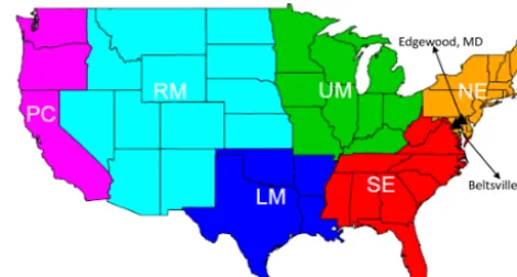
Figure 1. Analysis regions and ozonesonde locations during the 2011 DISCOVER-AQ field study.
and Pickering, 2014; Anderson et al., 2014; Follette-Cook et al., 2015) were used. During this campaign, the NASA P-3B aircraft measured trace gases including O3, NO, and NO2. Vertical profiles were obtained over seven locations – Beltsville (Be), Padonia (Pa), Fair Hill (Fa), Aldino (Al), Edgewood (Ed), Essex (Es), and Chesapeake Bay (Cb) from approximately 0.3 to 5 km above ground level during P-3B flights over 14 d in July 2011. During this same period, ozonesonde measurements were taken that extended from ground level through the entire model column at two lo-cations (Beltsville, MD, and Edgewood, MD, as shown in Fig. 1). Inclusion of LNO estimates in the CTM simula-tions also has an important impact on model estimated wet deposition of nitrate. Therefore, assessment was also per-formed using data from the National Atmospheric Depo-sition Program’s National Trends Network (NADP NTN, http://nadp.slh.wisc.edu/ntn, last access: 2 October 2019).
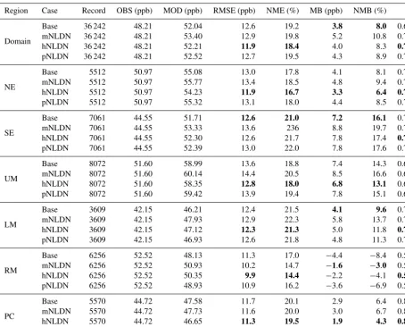
Table 1.Statistics of DM8HR O3for all model cases over the domain and analysis regions in July 2011. The best performance metrics among the model cases are highlighted in bold.
Region Case Record OBS (ppb) MOD (ppb) RMSE (ppb) NME (%) MB (ppb) NMB (%) R
Domain
Base 36 242 48.21 52.04 12.6 19.2 3.8 8.0 0.69
mNLDN 36 242 48.21 53.40 12.9 19.8 5.2 10.8 0.70
hNLDN 36 242 48.21 52.21 11.9 18.4 4.0 8.3 0.72
pNLDN 36 242 48.21 52.52 12.7 19.5 4.3 8.9 0.70
NE
Base 5512 50.97 55.08 13.0 17.8 4.1 8.1 0.74
mNLDN 5512 50.97 55.77 13.4 18.5 4.8 9.4 0.74
hNLDN 5512 50.97 54.23 11.9 16.7 3.3 6.4 0.75
pNLDN 5512 50.97 55.32 13.1 18.0 4.4 8.5 0.74
SE
Base 7061 44.55 51.71 12.6 21.0 7.2 16.1 0.76
mNLDN 7061 44.55 53.33 13.6 236 8.8 19.7 0.76
hNLDN 7061 44.55 52.30 12.6 21.7 7.8 17.4 0.77
pNLDN 7061 44.55 52.39 13.0 22.0 7.8 17.6 0.76
UM
Base 8072 51.60 58.99 13.6 18.8 7.4 14.3 0.64
mNLDN 8072 51.60 60.14 14.4 20.5 8.5 16.6 0.64
hNLDN 8072 51.60 58.35 12.8 18.0 6.8 13.1 0.64
pNLDN 8072 51.60 59.42 13.9 19.4 7.8 15.1 0.64
LM
Base 3609 42.15 46.21 12.4 21.5 4.1 9.6 0.73
mNLDN 3609 42.15 47.93 12.9 22.3 5.8 13.7 0.74
hNLDN 3609 42.15 47.12 12.3 21.3 5.0 11.8 0.76
pNLDN 3609 42.15 46.93 12.6 21.8 4.8 11.3 0.74
RM
Base 6256 52.52 48.13 11.3 17.0 −4.4 −8.4 0.52
mNLDN 6256 52.52 50.93 10.2 14.7 −1.6 −3.0 0.56
hNLDN 6256 52.52 50.35 9.9 14.4 −2.2 −4.1 0.57
pNLDN 6256 52.52 48.93 10.9 16.2 −3.6 −6.9 0.53
PC
Base 5570 44.72 47.58 11.7 20.1 2.9 6.4 0.80
mNLDN 5570 44.72 47.73 11.6 20.0 3.0 6.7 0.80
hNLDN 5570 44.72 46.65 11.3 19.5 1.9 4.3 0.81
pNLDN 5570 44.72 47.62 11.6 20.0 2.9 6.5 0.80
3 Results
3.1 Ground-level evaluation for O3and NOx
3.1.1 Statistical performance metrics
Tables 1 and 2 display the statistical model performance met-rics for daily maximum 8 h (DM8HR) O3 and daily mean NOx mixing ratios over the domain and each analysis
re-gion for all four model cases in July 2011 (Base, mNLDN, hNLDN, and pNLDN). The best performance metrics among the model cases are highlighted in bold. As shown in Table 1, for DM8HR O3, the Base simulation has the lowest MB and NMB values over the domain, while hNLDN produced the smallest RMSE and NME values. The mNLDN generated the largest values for both error (RMSE and NME) and biases (MB and NMB), followed by pNLDN, and all model cases with LNO exhibit slightly higher correlation coefficients than the Base simulation. Additionally, the hNLDN simulation exhibited higher correlation and lower bias and error relative
to the measurements indicating the value of higher-temporal-resolution lightning activity for representing the associated NOxemissions and their impacts on tropospheric chemistry.
Examining the regional results for DM8HR O3in Table 1, the statistical measures indicate that in the northeast (NE), hNLDN outperformed all other model cases with the lowest errors and biases and highest correlation coefficient. In the southeast (SE), the Base simulation performed better with the lowest errors and mean biases, but the correlation coefficient (R) value for hNLDN is slightly higher. Among all the LNO cases, mNLDN produced the worst statistics in this region. Historically, CTMs tend to significantly overestimate surface O3 in the southeast US (Lin et al., 2008; Fiore et al., 2009; Brown-Steiner et al., 2015; Canty et al., 2015), and this is partially driven by a likely overestimation of anthropogenic NOx emissions (Anderson et al., 2014). Thus, even though
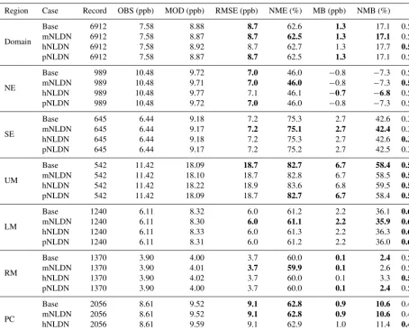
Table 2.Statistics of daily mean NOxfor all model cases over the domain and analysis regions in July 2011. The best performance metrics among the model cases are highlighted in bold.
Region Case Record OBS (ppb) MOD (ppb) RMSE (ppb) NME (%) MB (ppb) NMB (%) R
Domain
Base 6912 7.58 8.88 8.7 62.6 1.3 17.1 0.54
mNLDN 6912 7.58 8.87 8.7 62.5 1.3 17.1 0.54
hNLDN 6912 7.58 8.92 8.7 62.7 1.3 17.7 0.55
pNLDN 6912 7.58 8.87 8.7 62.5 1.3 17.1 0.54
NE
Base 989 10.48 9.72 7.0 46.0 −0.8 −7.3 0.55
mNLDN 989 10.48 9.71 7.0 46.0 −0.8 −7.3 0.55
hNLDN 989 10.48 9.77 7.1 46.1 −0.7 −6.8 0.55
pNLDN 989 10.48 9.72 7.0 46.0 −0.8 −7.3 0.55
SE
Base 645 6.44 9.18 7.2 75.3 2.7 42.6 0.34
mNLDN 645 6.44 9.17 7.2 75.1 2.7 42.4 0.34
hNLDN 645 6.44 9.18 7.2 75.3 2.7 42.6 0.34
pNLDN 645 6.44 9.17 7.2 75.2 2.7 42.5 0.34
UM
Base 542 11.42 18.09 18.7 82.7 6.7 58.4 0.58
mNLDN 542 11.42 18.10 18.7 82.8 6.7 58.5 0.58
hNLDN 542 11.42 18.22 18.9 83.6 6.8 59.5 0.58
pNLDN 542 11.42 18.09 18.7 82.7 6.7 58.4 0.58
LM
Base 1240 6.11 8.32 6.0 61.2 2.2 36.1 0.68
mNLDN 1240 6.11 8.30 6.0 61.1 2.2 35.9 0.68
hNLDN 1240 6.11 8.33 6.0 61.3 2.2 36.3 0.68
pNLDN 1240 6.11 8.31 6.0 61.2 2.2 36.0 0.68
RM
Base 1370 3.90 4.00 3.7 60.0 0.1 2.4 0.58
mNLDN 1370 3.90 4.01 3.7 59.9 0.1 2.6 0.58
hNLDN 1370 3.90 4.02 3.7 60.0 0.1 3.3 0.58
pNLDN 1370 3.90 4.00 3.7 60.0 0.1 2.4 0.58
PC
Base 2056 8.61 9.52 9.1 62.8 0.9 10.6 0.48
mNLDN 2056 8.61 9.52 9.1 62.8 0.9 10.6 0.48
hNLDN 2056 8.61 9.59 9.1 62.9 1.0 11.4 0.48
pNLDN 2056 8.61 9.52 9.1 62.8 0.9 10.6 0.48
the modeling system. As noted in Table 1, compared to the Base, the MB values in the SE increased by about 1.6 ppb with mNLDN and increased by less than 1 ppb with hNLDN and pNLDN. Nevertheless, the correlation coefficients for mNLDN and pNLDN were almost the same with the Base, and hNLDN was slightly higher (0.77 compared to 0.76). These correlations indicate that even though additional NOx
increases the mean bias, when it is added correctly in time and space, as with the case of hNLDN, the spatial and tempo-ral correlation are slightly improved. In the Upper Midwest (UM), the lowest errors and biases among the model cases are associated with hNLDN, while the worst performance is with mNLDN. In the Lower Midwest (LM), hNLDN per-formed comparable with the Base, with hNLDN having the highest correlation and lowest mean errors, while the Base has the lowest mean biases. The Rocky Mountain (RM) re-gion is the only rere-gion that shows an underestimation of DM8HR O3. In this region all the model cases with LNO out-performed the Base case in all the metrics. Among the three
model cases with LNO, mNLDN produced the lowest MB and NMB values, while hNLDN had the lowest RMSE and NME, and the highest correlation. In the Pacific Coast (PC) region, lightning activity is generally very low compared to other regions (Kang and Pickering, 2018). All model cases with LNO outperformed the Base case, especially hNLDN which had the lowest mean error and bias and highest corre-lation among all the cases.
Most of the NOx produced by lightning is distributed in
the middle and upper troposphere with only a small portion being distributed close to the surface. As a result, the impact on ground-level NOxmixing ratios is small. Table 2 shows
all the model cases produced similar statistics for the daily mean NOxmixing ratios at AQS sites across the domain and
Figure 2. Time series of regional-mean daily maximum 8 h O3 comparing observations (AQS) and CMAQ model predictions us-ing the LNOx schemes to Base simulation for the domain(a), for SE(b), and for RM(c)in July 2011. The numbers in the parentheses following the region names are the number of AQS sites.
3.1.2 Time series
Figure 2 presents time series of regional-mean observed and modeled DM8HR O3 for the entire domain and the SE and RM regions during July 2011. Over the domain and in SE, all the model cases overestimate the mean DM8HR O3mixing ratios on all days with the Base being the closest to the ob-servations. The hNLDN is almost the same as the Base with slightly higher values on some days. Among all the cases, mNLDN produced the highest values on almost all days through the month, on the order of 1–2 ppb higher than the Base. In contrast, in the RM region, the Base significantly un-derestimates DM8HR O3mixing ratios on all the days during the month, while all model cases with LNO improved model predictions relative to observations in the region. Among the three model cases with LNO, mNLDN produced the lowest bias for all the days, closely followed by hNLDN.
Figure 3.Time series of daily mean NOxover the domain(a), SE
(b), and RM(c)in July 2011. The numbers in the parentheses fol-lowing the region names are the number of AQS sites.
Figure 3 displays the average daily mean NOxmixing
ra-tios at AQS sites over the same regions as in Fig. 2. On most of the days in July 2011, over the domain and in the SE, the model overestimate NOx values, and on almost half of the
days the overestimation is significant (up to 100 %). As noted in Table 2, on average, the overestimation is∼17 % over the domain and∼43 % in SE. However in RM, the predicted NOxmixing ratios closely follow the daily observations and
on average the modeled and observed magnitude is almost identical (∼3 % difference). All the model cases, with or without LNO, produced almost the same mean NOx mixing
Figure 4.Diurnal profiles for hourly O3and NOxover the domain(a, d), SE(b, e), and RM(c, f)in July 2011.
3.1.3 Diurnal variations
Diurnal plots are used to further examine differences in model evaluation for O3and NOx. Figure 4 shows the mean
diurnal profiles for hourly O3and NOx over the entire
do-main, SE, and RM. On a domain mean basis, all model cases overestimate O3 during the daytime hours, while in the SE the overestimation spans all the hours. In RM, the model cases significantly underestimate O3across all the hours ex-cept for a few early morning hours, when the model pre-dicted values are very close to the observations. Among all the model cases, as expected, the most prominent differences occurred during the midday hours when the photochemistry is most active. However, the difference between hNLDN (and mNLDN) and the Base is also significant during the night in the RM region, even though the O3 levels are low. This may be attributed to NOx-related nighttime chemistry in part
caused by freshly released NO by cloud-to-ground lightning
flashes. The diurnal variations of NOx are similar over the
domain and in the regions for all model cases. Appel et al. (2017) reported a significant overestimation of NOx
mix-ing ratios at AQS sites durmix-ing nighttime hours and underes-timation during daytime hours. The bias pattern is identical for all of the LNO model cases evaluated here (Fig. 4).
3.1.4 Spatial variations
Figure 5 shows the impact of the different LNO schemes on model performance for DM8HR O3at AQS sites. The spatial maps show the difference in absolute MB between the cases with lightning NOxemissions and the Base and is calculated
Figure 5.Spatial maps of the mean bias of DM8HR O3(model – observation) differences between model case with LNOxand the Base as well as the corresponding histograms indicating the number of sites with decreased mean bias for each pair of model cases in July 2011.
Figure 6. Vertical profiles of O3 mixing ratios from ozonesonde measurements and model simulations at Beltsville, MD (a); and Edgewood, MD,(b)on the days when lightning NO produced sig-nificant impact on O3 during the DISCOVER-AQ field study in July 2011.
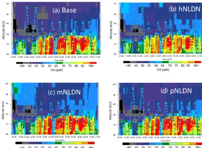
Figure 7.Overlay of P-3B-observed O3(1 min mean values) over the corresponding vertical cross sections of simulated values extracted at the flying locations on 28 July 2018,(a)Base,(b)hNLDN(c)mNLDN, and(d)pNLDN. The letters marked at the bottom of the plots are P-3B spiral sites, Be: Beltsville, Pa: Padonia, Fa: Fair Hill, Al: Aldino, Ed: Edgewood, and Es: Essex.
3.2 Vertical evaluation for O3and NOx
3.2.1 Ozone-sonde observations
A large source of uncertainty in the specification of LNO is its vertical allocation, which can impact the model’s ability to accurately represent the variability in both chemistry and transport. To further assess the impact of the vertical LNO specification on model results, we compared vertical profiles of simulated model O3with extensive ozonesonde measure-ments available during the study period. Figure 6 presents the vertical profiles for O3 sonde measurements and paired model estimates of all model cases at Beltsville, MD, and Edgewood, MD. At each location, observations from multi-ple days are available (one or two soundings per day) dur-ing the 2011 DISCOVER-AQ campaign in July 2011. The model evaluation was limited to days where the inclusion of LNO has an obvious impact (the mean vertical profiles of LNO cases are separable from that of the Base case) on the model estimates (21, 22, 28, and 29 July at Beltsville, and 21, 22, 28, 29, and 30 July at Edgewood). We paired the ob-served data with model estimates in time and space and av-eraged the model and observed values at each model layer. Only data below 12 km altitude are plotted in Fig. 6 to ex-clude possible influence of stratospheric air on O3. As can be
seen in Fig. 6, at both locations the Base case underestimates O3mixing ratios above about 1 km, but overestimates values closer to the surface. When LNO is included in the simu-lations, the predicted O3 mixing ratios increase relative to the Base case starting around 2 km, with greater divergence from the Base case at higher altitudes. The two model cases, hNLDN and mNLDN, produced similar O3levels from the surface to about 6 km, but above that altitude the mNLDN ozone mixing ratios were higher. All the model cases with LNO performed much better aloft than the Base case. Near the surface, all the model cases overestimated O3, however hNLDN had smaller bias than the other simulations. This may be attributed to the fact that only hNLDN used the ob-served lightning flash data directly, and as a result, LNO was estimated more accurately in time and space. This improve-ment in model bias at the surface is further investigated in the next section using evaluation against P-3B measurements.
3.2.2 P-3B measurement
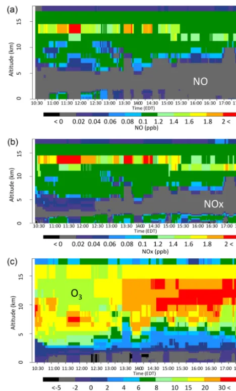
Figure 8.The vertical-time difference between hNLDN and Base during the P-3B flight period on 28 July 2011 for(a)NO,(b)NOx, and(c)O3.
mean vertical profiles of LNO cases are separable from that of the Base case) lightning impacts, to evaluate the model simulations. Figure 7 shows measured O3mixing ra-tios overlaid on the modeled vertical time section for 10:30– 17:30 UTC. The color-filled circles represent measured O3 mixing ratios averaged over 60 s and the background is the model estimated vertical profiles from the grid cells contain-ing the P-3B flight path for that hour and location. As indi-cated in the Base case (Fig. 7a), the model tends to overesti-mate O3mixing ratios from the surface to about 2 km, but it tends to underestimate at altitudes above 2 km. The hNLDN reduced the overestimation below 2 km, e.g., fewer grid cells with mixing ratios above 90 ppb (shown in red). The other two cases (mNLDN and pNLDN) did not produce the same improvement near the surface. The hNLDN also decreases the underestimation aloft compared to the Base case with O3 mixing ratios in the 55–65 ppb range (light blue colors),
bet-Figure 9.The vertical-time difference between mNLDN and Base during the P-3B flight period on 28 July 2011 for(a)NO,(b)NOx, and(c)O3.
ter matching the measured values. This decrease in underes-timation aloft is also seen in the mNLDN case, but to a lesser degree while the pNLDN case shows only slight improve-ment aloft over the Base simulation.
To further differentiate the three LNO model cases, Figs. 8–10 show the difference in the time sections between each of the model cases with LNO and the Base for NO, NOx, and O3from all the model layers along the P-3B flight path on 28 July. As seen in Fig. 8, the hNLDN scheme in-jected most NO above 5 km with a peak between 13 and 14 km and only a small amount near the surface. After re-lease into the atmosphere, NO is quickly converted into NO2 in the presence of O3, and these collectively result in the NOx vertical time section (local production plus transport)
shown in the middle panel of Fig. 8. NOx is further mixed
sig-Figure 10.The vertical-time difference between pNLDN and Base during the P-3B flight period on 28 July 2011 for(a)NO,(b)NOx, and(c)O3.
nificant O3 is produced above 3 km, and the maximum O3 difference appears between 9 and 14 km during the early af-ternoon hours (from 13:30 to 17:30 Eastern Daylight Time). However, from surface to about 2 km, O3 is reduced con-sistently across the entire period, and this is the result of O3 titration by NO from cloud-to-ground lightning flashes that must have been transported to this layer by storm down-drafts. Since O3is significantly underestimated above 3 km and overestimated near the surface by the Base model, the inclusion of LNO greatly improved the model’s performance under both conditions.
Comparison of Fig. 9 (mNLDN) with Fig. 8 (hNLDN) re-veals that the time sections of NO and NOxare similar above
5 km but dramatically different near the surface. The near-surface increase in ambient NO noted in the hNLDN is ab-sent in mNLDN, and in fact there are some small decreases in NO, although the reason for this is unclear. The increase in O3aloft in the mNLDN case is similar to that seen in the
Figure 11.Bias (model – observation) distributions of O3(a)and NO(b)at each P-3B spiral site on 21, 22, 28, and 29 July 2011. Be: Beltsville, Pa: Padonia, Fa: Fair Hill, Al: Aldino, Ed: Edgewood, Es: Essex, and Cb: Chesapeake Bay.
hNLDN case. However, the near-surface reduction in O3is almost absent. In the pNLDN case (Fig. 10), NO mixing ra-tios are much less than those in hNLDN and mNLDN in the upper layers as a result of less column NO being generated by the linear parameterization. The resulting NOx time section
is also smoothed. The pNLDN time sections for NO, NOx,
and O3near the surface are similar to the mNLDN case with no change or small decreases compared to the Base case. O3 mixing ratios increase by more than 30 ppb during the after-noon hours between 10 and 13 km in the pNLDN case, how-ever the increase is not as intense and widespread as the other cases. In summary, the hNLDN scheme produces estimates that are more consistent with measurements at the surface and aloft, compared to the other simulations, reflecting the advantage of using the spatially and temporally resolved ob-served lightning flash data. The model performance improve-ment for simulated O3distributions also suggests robustness in the vertical distribution scheme when LNO is generated at the right time and location.
Figure 12. (a)–(c)shows precipitation estimates from WRF(a), the bias in the WRF predicted precipitation at NTN locations(b), and the corresponding scatter plots(c).(d)–(f)shows wet deposition (dep) of nitrate estimates from the Base simulation(d), the bias in the Base model estimates of wet deposition of NO−3 at NADP NTN locations(e), and the corresponding scatter plots(f).(g)–(i)shows the difference in the LNOxsensitivity simulations and the Base case estimates of wet deposition of NO−3 for mNLDN – Base(g); hNLDN – Base(h), and pNLDN – Base(i). All maps are based on accumulated values (precipitation or wet deposition) during June–August 2011. Precipitation totals are in centimeters (cm) and wet deposition totals are in kilograms per hectare (kg ha−1).
in all cases, the lightning NO was injected approximately 200 km upwind (northwest) of the flight path. The hNLDN case captured two injections: one occurred during the morn-ing hours (05:00 to 07:00 EDT) and the other happened dur-ing the afternoon hours (after 02:30 EDT). Both mNLDN and pNLDN captured the afternoon lightning event at the later time (after 03:30 EDT for mNLDN and after 04:30 for pNLDN) with varying intensity, but neither captured the morning lightning event, which explains why the increase in NO and NOxin the hNLDN case (Fig. 8) did not occur in the
mNLDN and pNLDN cases (Figs. 9 and 10). Also note that the significant increase of NO during the time period from 11:00 to 13:00 EDT occurred about 5 h after the lightning NO was injected at about 200 km upwind in the hNLDN case.
To expand on the evaluation in Figs. 7–10 which focused on measurements from 28 July 2011, we retrieved all the P-3B measurements on days with noticeable lightning impact
(21, 22, 28, and 29 July). The 3-D paired observation–model data were grouped together by spiral site and the mean biases (model – observation) were plotted in Fig. 11 (a and b) for O3 and NO, respectively. The boxplots for O3in Fig. 11a sug-gests that the Base exhibited larger bias with greater spread (i.e., larger interquartile range) than other model cases incor-porating LNO at most of the locations where aircraft spirals were conducted. At all locations except Aldino, the lowest mean biases in simulated NO and O3are noted in the hNLDN simulation.
3.3 Deposition evaluation for nitrate
In addition to contributing to tropospheric O3 formation, NOx oxidation also leads to gaseous nitric acid and
im-Table 3.Statistics of June–August 2011 accumulated precipitation (cm) and wet deposition of nitrate (NO−3) for all model cases over the domain. The best performance metrics among the model cases are highlighted in bold.
OBS MOD RMSE NME MB NMB
Region Case Record (cm, kg ha−1) (cm, kg ha−1) (cm, kg ha−1) (%) (cm, kg ha−1) (%) R
Domain
precip 196 24.8 23.9 7.5 23 −0.9 −4 0.87
Base 196 2.34 1.52 1.1 38 −0.8 −35 0.84
mNLDN 196 2.34 1.98 0.8 26 −0.4 −15 0.86
hNLDN 196 2.34 1.95 0.8 26 −0.4 −17 0.86
pNLDN 196 2.34 1.68 1.0 33 −0.7 −28 0.85
NE
precip 31 38.6 35.9 9.5 19 −2.7 −7 0.79
Base 31 2.96 2.32 1.1 29 −0.6 −23 0.70
mNLDN 31 2.96 2.71 0.9 24 −0.3 −8 0.76
hNLDN 31 2.96 2.74 0.9 24 −0.2 −7 0.74
pNLDN 31 2.96 2.48 1.0 27 −0.5 −16 0.73
SE
precip 39 36.1 31.7 9.4 21 −4.3 −12 0.80
Base 39 3.05 2.09 1.2 35 −1.0 −32 0.51
mNLDN 39 3.05 2.97 0.8 21 −0.1 −2 0.56
hNLDN 39 3.05 2.82 0.9 23 −0.2 −8 0.53
pNLDN 39 3.05 2.43 1.0 27 −0.6 −20 0.54
UM
precip 45 28.8 26.1 6.8 20 −2.7 −9 0.51
Base 45 3.17 1.98 1.4 38 −1.2 −38 0.73
mNLDN 45 3.17 2.51 0.9 24 −0.7 −21 0.77
hNLDN 45 3.17 2.48 0.9 25 −0.7 −22 0.77
pNLDN 45 3.17 2.15 1.2 33 −1.0 −32 0.76
LM
precip 12 12.3 10.4 4.1 29 −2.0 −16 0.90
Base 12 1.44 0.85 0.7 41 −0.6 −41 0.90
mNLDN 12 1.44 1.16 0.6 33 −0.3 −19 0.88
hNLDN 12 1.44 1.13 0.6 32 −0.3 −21 0.89
pNLDN 12 1.44 0.93 0.7 36 −0.5 −35 0.88
RM
precip 50 13.7 18.2 6.9 39 4.4 32 0.91
Base 50 1.63 0.8 1.0 51 −0.8 −51 0.90
mNLDN 50 1.63 1.1 0.7 34 −0.5 −32 0.91
hNLDN 50 1.63 1.12 0.7 33 −0.5 −31 0.90
pNLDN 50 1.63 0.86 1.0 48 −0.8 −47 0.91
PC
precip 19 7.01 6.53 2.4 29 −0.48 −6.8 0.84
Base 19 0.31 0.31 0.18 44 0.00 −1.0 0.88
mNLDN 19 0.31 0.33 0.19 48 0.01 3.9 0.89
hNLDN 19 0.31 0.33 0.20 50 0.02 6.6 0.89
pNLDN 19 0.31 0.31 0.18 44 0.00 −0.3 0.88
portant role in nitrogen deposition modeling. To assess the impacts of incorporating LNO emissions on simulated ox-idized nitrogen deposition, we compared model estimated amounts of precipitation from the NTN network (http://nadp. slh.wisc.edu/ntn/, last access: 2 October 2019) and wet depo-sition of NO−3 with measurements from the NADP network (http://nadp.slh.wisc.edu/, last access: 2 October 2019). Dur-ing summer months in 2011 (June–August) the WRF model generally reproduces the observed precipitation with a slight underestimate in the east, but the Base model simulation tends to underestimate wet deposition of NO−3 across the do-main, with the greatest underestimation in the SE and UM
most LNO among the three LNO schemes, thus it results in the smallest errors in terms of wet deposition of NO−3 when compared to the Base simulation that significantly underes-timated NO−3 wet deposition. It should be noted that in ad-dition to the LNO contributions, errors in modeled precipita-tion amounts and patterns also likely influence the underesti-mation of NO−3 wet deposition.
4 Conclusions
A detailed evaluation of lightning NOx emission estimation
parameterizations available in the CMAQ modeling system was performed through comparisons of model simulation re-sults with surface and aloft air quality measurements.
Our analysis indicates that incorporation of LNO emis-sions enhanced O3production in the middle and upper tro-posphere, where O3 mixing ratios were often significantly underestimated without the representation of LNO. Though the impact on surface O3 varies from region to region and is also dependent on the accuracy of the NOx emissions
from other sources, the inclusion of LNO, when it is in-jected at the appropriate time and location, can improve the model estimates. In regions where the Base model estimates of O3 were biased high, the inclusion of LNO further in-creased the model bias, and a systematic increase is noted in the correlation with measurements, suggesting that emissions from other sources likely drive the overestimation. Identify-ing how errors in emission inputs from different sources in-teract with errors in meteorological modeling of mixing and transport remains a challenging but critical task. Likewise, all the LNO schemes also enhanced the accumulated wet de-position of NO−3 that was significantly underestimated by the Base model without LNO throughout the modeling domain except the Pacific Coast.
Uncertainty remains in modeling the magnitude and spa-tial, temporal, and vertical distribution of lightning produced NOx. LNO schemes are built on numerous assumptions and
all current schemes also depend on the skill of the up-stream meteorological models in describing convective activ-ity. Nevertheless, these schemes reflect our best understand-ing and knowledge at the time when the schemes were im-plemented. The use of hourly information on lightning ac-tivity yielded LNO emissions that generally improved model performance for ambient O3 and NOx as well as oxidized
nitrogen wet deposition amounts. As more high-quality data from both ground and satellite measurements become avail-able, the performance of the LNO schemes will continue to improve.
Since the pNLDN scheme was developed using historical data correlating lightning activity with convective precipita-tion, the scheme could be employed for applications involv-ing air quality forecastinvolv-ing and future projections when ob-served lightning information is not available.
Code and data availability. CMAQ model documentation and re-leased versions of the source code, including all model code used in his study, are available at https://doi.org/10.5281/zenodo.1167892 (US EPA Office of Research and Development, 2017).
The data processing and analysis scripts are available upon re-quest. The WRF model is available for download through the WRF website (http://www2.mmm.ucar.edu/wrf/users/wrfv3.8/updates-3. 8.html, last access: 2 October 2019; NCAR, 2018).
The raw lightning flash observation data used are not available to the public but can be purchased through Vaisala Inc. (https:// www.vaisala.com/en/products/systems/lightning-detection, last ac-cess: 2 October 2019; Vaisala, 2019). The lightning data obtained from Vaisala Inc. is the cloud-to-ground lightning flashes over the contiguous United States. The immediate data behind the tables and figures are available from https://zenodo.org/record/3360744 (last access: 2 October 2019; Kang and Foley, 2019). Additional input and output data for CMAQ model utilized for this analysis are also available upon request.
Author contributions. DK collected the data, designed the algo-rithm, performed the model simulation, carried out the analysis, and wrote the paper. KF performed the data analysis and was involved in the writing of the paper. RM, SR, KP, and DA edited the paper.
Competing interests. The authors declare that they have no conflict of interest.
Disclaimer. The views expressed in this paper are those of the au-thors and do not necessarily represent the views or policies of the U.S. EPA.
Acknowledgements. The authors thank Brian Eder, Golam Sarwar, and Janet Burke (U.S. EPA) for their constructive comments and suggestions during the internal review process.
Review statement. This paper was edited by Slimane Bekki and re-viewed by two anonymous referees.
References
Allen, D. J. and Pickering, K. E.: Evaluation of lightning flash rate parameterizations for use in a global chemi-cal transport model, J. Geophys. Res., 107, 4711–4731, https://doi.org/10.1029/2002JD002066, 2002.
Allen, D., Pickering, K., Stenchikov, G., Thompson, A., and Kondo, Y.: A three-dimensional total odd nitrogen (NOy) simulation during SONEX using a stretched-grid chemi-cal transport model, J. Geophys. Res., 105, 3851–3876, https://doi.org/10.1029/1999JD901029, 2000.
determined using the CMAQ model, Atmos. Chem. Phys., 12, 1737–1758, https://doi.org/10.5194/acp-12-1737-2012, 2012. Anderson, D. C., Loughner, C. P., Diskin, G., Weinheimer, A.,
Canty, T. P., Salawitch, R. J, Worden, H. M., Fried, A., Mikoviny, T., Wisthaler, A., and Dickerson, R. R.: Measured and modeled CO and NOy in DISCOVER-AQ: An evaluation of emissions and chemistry over the eastern US, Atmos. Environ., 96, 78–87, https://doi.org/10.1016/j.atmosenv.2014.07.004, 2014.
Appel, K. W., Foley, K. M., Bash, J. O., Pinder, R. W., Dennis, R. L., Allen, D. J., and Pickering, K.: A multi-resolution assessment of the Community Multiscale Air Quality (CMAQ) model v4.7 wet deposition estimates for 2002–2006, Geosci. Model Dev., 4, 357–371, https://doi.org/10.5194/gmd-4-357-2011, 2011. Appel, K. W., Napelenok, S. L., Foley, K. M., Pye, H. O., Hogrefe,
C., Luecken, D. J., Bash, J. O., Roselle, S. J., Pleim, J. E., Foroutan, H., Hutzell1, W. D., Pouliot, G. O., Sarwar, G., Fahey, K. M., Gantt, G., Gilliam, R. C., Heath, N. K., Kang, D., Mathur, R., Schwede, D. B., Spero, T. L., Wong, D. C., and Young, J. O.: Description and evaluation of the Community Multi-scale Air Quality (CMAQ) modeling system version 5.1, Geosci. Model Dev., 10, 1703–1732, https://doi.org/10.5194/gmd-10-1703-2017, 2017.
Bash, J. O., Baker, K. R., and Beaver, M. R.: Evaluation of improved land use and canopy representation in BEIS v3.61 with biogenic VOC measurements in California, Geosci. Model Dev., 9, 2191– 2207, https://doi.org/10.5194/gmd-9-2191-2016, 2016.
Bovensmann, H., Burrows, J. P., Buchwitz, M., Frerick, J., Noël, S., Rozanov, V. V., Chance, K. V., and Goede, A. P. H.: SCIA-MACHY: Mission Objectives and Measurement Modes, J. At-mos. Sci., 56, 127–150, 1999.
Brown-Steiner, B., Hess, P. G., and Lin, M. Y.: On the capabilities and limitations of GCCM simulations of summertime regional air quality: A diagnostic analysis of ozone and temperature sim-ulations in the US using CESM CAM-Chem, Atmos. Environ., 101, 134–148, https://doi.org/10.1016/j.atmosenv.2014.11.001, 2015.
Byun, D. W. and Schere, K. L.: Rewiew of the governing equations, computational algorithms, and other components of the Models-3 Community Multiscale Air Quality (CMAQ) modeling system, Appl. Mech. Rev., 59, 51–77, 2006.
Canty, T. P., Hembeck, L., Vinciguerra, T. P., Anderson, D. C., Goldberg, D. L., Carpenter, S. F., Allen, D. J., Loughner, C. P., Salawitch, R. J., and Dickerson, R. R.: Ozone and NOx chemistry in the eastern US: evaluation of CMAQ/CB05 with satellite (OMI) data, Atmos. Chem. Phys., 15, 10965–10982, https://doi.org/10.5194/acp-15-10965-2015, 2015.
Choi, Y., Wang, Y., Zeng, T., Martin, R. V., Kurosu, T. P., and Chance, K.: Evidence of lightning NOx and con-vective transport of pollutants in satellite observations over North America, Geophys. Res. Lett., 32, L02805, https://doi.org/10.1029/2004GL021436, 2005.
Crawford, J. H. and Pickering, K. E.: DISCOVER-AQ: Advancing strategies for air quality observations for the next decade, EM, A&WMA, September, 2014.
Eder, B. K., Kang, D., Mathur, R., Yu, S., and Schere, K.: An oper-ational evaluation of the Eta-CMAQ air quality forecast model, Atmos. Environ., 40, 4894–4905, 2006.
Finney, D. L., Doherty, R. M., Wild, O., Huntrieser, H., Pumphrey, H. C., and Blyth, A. M.: Using cloud ice flux to parametrize
large-scale lightning, Atmos. Chem. Phys., 14, 12665–12682, https://doi.org/10.5194/acp-14-12665-2014, 2014.
Finney, D. L., Doherty, R. M., Wild, O., and Abraham, N. L.: The impact of lightning on tropospheric ozone chemistry using a new global lightning parameterization, Atmos. Chem. Phys., 16, 7507–7522, https://doi.org/10.5194/acp-16-7507-2016, 2016. Fiore, A. M., Dentener, F. J., Wild, O., Cuvelier, C., Schultz, M.
G., Hess, P., Textor, C., Schulz, M., Doherty, R. M., Horowitz, L. W., MacKenzie, I. A., Sanderson, M. G., Shindell, D. T., Steven-son, D. S., Szopa, S., Van Dingenen, R., Zeng, G., Atherton, C., Bergmann, D., Bey, I., Carmichael, G., Collins, W. J., Duncan, B. N., Faluvegi, G., Folberth, G., Gauss, M., Gong, S., Hauglus-taine, D., Holloway, T., Isaksen, I. S. A., Jacob, D. J., Jonson, J. E., Kaminski, J. W., Keating, T. J., Lupu, A., Marmer, E., Montanaro, V., Park, R. J., Pitari, G., Pringle, K. J., Pyle, J. A., Schroeder, S., Vivanco, M. G., Wind, P., Wojcik, G., Wu, S., and Zuber, A.: Multimodel estimates of intercontinental sourcere-ceptor relationships for ozone pollution, J. Geophys. Res., 114, D04301, https://doi.org/10.1029/2008jd010816, 2009.
Flatoy, F. and Hov, O.: NOx from lightning and the calculated chemical composition of the free troposphere, J. Geophys. Res.-Atmos., 102, 21373–21381, https://doi.org/10.1029/97JD01308, 1997.
Foley, K. M., Roselle, S. J., Appel, K. W., Bhave, P. V., Pleim, J. E., Otte, T. L., Mathur, R., Sarwar, G., Young, J. O., Gilliam, R. C., Nolte, C. G., Kelly, J. T., Gilliland, A. B., and Bash, J. O.: Incremental testing of the Community Multiscale Air Quality (CMAQ) modeling system version 4.7, Geosci. Model Dev., 3, 205–226, https://doi.org/10.5194/gmd-3-205-2010, 2010. Follette-Cook, M. B., Pickering, K. E., Crawford, J. H.,
Duncan, B. N., Loughner, C. P., Diskin, G. S., Fried, A., and Weinheimer, A. J.: Spatial and temporal variabil-ity of trance gas columns derived from WRF/Chem re-gional model output: Planning for geostationary observations of atmospheric composition, Atmos. Environ., 118, 28–44, https://doi.org/10.1016/j.atmosenv.2015.07.024, 2015.
Kang, D. and Foley, K.: Simulating Lightning NO Pro-duction in CMAQv5.2: Performance Evaluations, data set, https://doi.org/10.5281/zenodo.3360744, 2019.
Kang, D. and Pickering, K. E.: Lightning NOxemissions and the Implications for Surface Air Quality over the Contiguous United States, EM, A&WMA, November, 2018.
Kang, D., Eder, B. K., Stein, A. F., Grell, G. A., Peckham, S. E., and Mchenry, J.: The New England air quality forecasting pilot pro-gram: development of an evaluation protocol and performance benchmark, J. Air Waste Manage. Assoc., 55, 1782–1796, 2005. Kang, D., Pickering, K. E., Allen, D. J., Foley, K. M., Wong, D., Mathur, R., and Roselle, S. J.: Simulating Lightning NO Pro-duction in CMAQv5.2: Evolution of Scientific Updates, Geosci. Model Dev., 12, 3071–3083, https://doi.org/10.5194/gmd-12-3071-2019, 2019.
Kaynak, B., Hu, Y., Martin, R. V., Russell, A. G., Choi, Y., and Wang, Y.: The effect of lightning NOx production on surface ozone in the continental United States, Atmos. Chem. Phys., 8, 5151–5159, https://doi.org/10.5194/acp-8-5151-2008, 2008. Koo, B., Chien, C. J., Tonnesen, G., Morris, R., Johnson,
emis-sions control strategies. Atmos Environ., 44, 2372–2382, https://doi.org/10.1016/j.atmosenv.2010.02.041, 2010.
Koshak, W., Peterson, H., Biazar, A., Khan, M., and Wang, L.: The NASA Lightning Nitrogen Oxides Model (LNOM): Appli-cation to air quality modeling, Atmos. Res., 135–136, 363–369, https://doi.org/10.1016/j.atmosres.2012.12.015, 2014.
Labrador, L. J., von Kuhlmann, R., and Lawrence, M. G.: The effects of lightning-produced NOx and its vertical dis-tribution on atmospheric chemistry: sensitivity simulations with MATCH-MPIC, Atmos. Chem. Phys., 5, 1815–1834, https://doi.org/10.5194/acp-5-1815-2005, 2005.
Lin, J., Youn, D., Liang, X., and Wuebbles, D.: Global model simulation of summertime U.S. ozone diurnal cycle and its sensitivity to PBL mixing, spatial reso-lution, and emissions, Atmos. Environ., 42, 8470–8483, https://doi.org/10.1016/j.atmosenv.2008.08.012, 2008.
Murray, L. T.: Lightning NOx and Impacts on Air Quality, Curr Pollution Rep., 2, 115–133, https://doi.org/10.1007/s40726-016-0031-7, 2016.
Napelenok, S. L., Pinder, R. W., Gilliland, A. B., and Martin, R. V.: A method for evaluating spatially-resolved NOx emissions using Kalman filter inversion, direct sensitivities, and space-based NO2 observations, Atmos. Chem. Phys., 8, 5603–5614, https://doi.org/10.5194/acp-8-5603-2008, 2008.
NCAR: WRF Model vrsion 3.8, updates, available at: http://www2. mmm.ucar.edu/wrf/users/wrfv3.8/updates-3.8.html (last access: 2 October 2019), 2018.
Nolte, C. G., Appel, K. W., Kelly, J. T., Bhave, P. V., Fahey, K. M., Collett Jr., J. L., Zhang, L., and Young, J. O.: Evaluation of the Community Multiscale Air Quality (CMAQ) model v5.0 against size-resolved measurements of inorganic particle com-position across sites in North America, Geosci. Model Dev., 8, 2877–2892, https://doi.org/10.5194/gmd-8-2877-2015, 2015. Novak, J. H. and Pierce, T. E.: Natural emissions of oxidant
precur-sors, Water Air Soil Poll., 67, 57–77, 1993.
Orville, R. E., Huffines, G. R., Burrows, W. R., Holle, R. L., and Cummins, K. L.: The North American Lightning Detection Net-work (NALDN) – first results: 1998–2000, Mon. Weather Rev., 130, 2098–2109, 2002.
Otte, T. L. and Pleim, J. E.: The Meteorology-Chemistry Inter-face Processor (MCIP) for the CMAQ modeling system: up-dates through MCIPv3.4.1, Geosci. Model Dev., 3, 243–256, https://doi.org/10.5194/gmd-3-243-2010, 2010.
Pickering, K. E., Bucsela, E., Allen, D., Ring, A., Holz-worth, R., and Krotkov, N.: Estimates of lightning NOx production based on OMI NO2 observations over the Gulf of Mexico, J. Geophys. Res.-Atmos., 121, 8668–8691, https://doi.org/10.1002/2015JD024179, 2016.
Price, C. and Rind, D.: A simple lightning parameterization for calculating global lightning distributions, J. Geophys. Res., 97, 9919–9933, https://doi.org/10.1029/92JD00719, 1992.
Price, C., Penner, J., and Prather, M.: NOxfrom lightning. 2. Con-straints from the global atmospheric electric circuit, J. Geo-phys. Res., 102, 5943–5951, https://doi.org/10.1029/96JD02551, 1997.
Richter, A., Burrows, J. P., Nüß, H., Granier, C., and Niemeier, U.: Increase in tropospheric nitrogen dioxide over China observed from space, Nature, 437, 129–132, https://doi.org/10.1038/nature04092, 2005.
Rossow, W. B., Walker, A. W., Beuschel, D. E., and Roiter, M. D.: International Satellite Cloud Climatology Project (ISCCP) doc-umentation of new cloud data sets, Tech. Rep. January, World Meteorological Organisation, WMO/TD 737, Geneva, 1996. Schumann, U. and Huntrieser, H.: The global lightning-induced
nitrogen oxides source, Atmos. Chem. Phys., 7, 3823–3907, https://doi.org/10.5194/acp-7-3823-2007, 2007.
Simon, H., Reff, A., Wells, B., Xing, J., and Frank, N.: Ozone trends across the United States over a period of decreasing NOx and VOC emissions. Environ. Sci. Technol., 49, 186–195, 2015. Sioris, C. E., Kurosu, T. P., Martin, R. V., and Chance, K.:
Strato-spheric and tropoStrato-spheric NO2observed by SCIAMACHY: first results, Adv. Space Res., 34, 780–785, 2004.
Smith, S. N. and Mueller, S. F.: Modeling natural emissions in the Community Multiscale Air Quality (CMAQ) Model-I: building an emissions data base, Atmos. Chem. Phys., 10, 4931–4952, https://doi.org/10.5194/acp-10-4931-2010, 2010.
Stockwell, D. Z., Giannakopoulos, C., Plantevin, P. H., Carver, G. D., Chipperfield, M. P., Law, K. S., Pyle, J. A., Shallcross, D. E., and Wang, K. Y.: Modelling NOxfrom lightning and its im-pact on global chemical fields, Atmos. Environ., 33, 4477–4493, 1999.
US EPA Office of Research and Development: CMAQ (Version 5.2), Zenodo, https://doi.org/10.5281/zenodo.1167892, 2017. Vaisala: Lightning Detection, available at: https://www.vaisala.
com/en/products/systems/lightning-detection, last access: 2 Oc-tober 2019.
Wang, L., Newchurch, M. J., Pour-Biazar, A., Kuang, S., Khan, M., Liu, X., Koshak, W., and Chance, K.: Estimating the influence of lightning on upper tropospheric ozone using NLDN lightning data and CMAQ model, Atmos. Environ., 67, 219–228, 2013. Yarwood, G., Whitten, G. Z., Jung, J., Heo, G., and Allen,