Advanced Multilinear Data Analysis and Sparse Representation Approaches and Their Applications

(1)

Advanced Multilinear Data Analysis and Sparse

Representation Approaches and Their Applications

Khoa Luu

A Thesis

In The Department of

Computer Science and Software Engineering

Presented in Partial Fulfillment of the Requirements

For the Degree of

Doctor of Philosophy in Computer Science

Concordia University

Montreal, Quebec, Canada

November 2013 © Khoa Luu, 2013.

(2)

CONCORDIA UNIVERSITY SCHOOL OF GRADUATE STUDIES This is to certify that the thesis prepared

By: Entitled:

and submitted in partial fulfillment of the requirements for the degree of

complies with the regulations of the University and meets the accepted standards with respect to originality and quality.

Signed by the final examining committee:

Chair External Examiner External to Program Examiner Examiner Thesis Supervisor Approved by Chair of Department or Graduate Program Director

Dean of Faculty

Khoa Luu

Advanced Multilinear Data Analysis and Sparse Representation Approaches and Their Applications

Doctor of Philosophy in Computer Science

Prof. Sudhir Mudur

Prof. Sri Krishnan (Ryerson University)

Prof. Adam Krzyzak

Prof. Wei-Ping Zhu

Profs. Tien D. Bui, Ching Y. Suen and Marios Savvides

(3)

iii

Advanced Multilinear Data Analysis and Sparse

Representation Approaches and Their Applications

Khoa Luu

Concordia University, 2013

Abstract

Multifactor analysis plays an important role in data analysis since most real-world datasets usually exist with a combination of numerous factors. These factors are usually not independent but interdependent together. Thus, it is a mistake if a method only considers one aspect of the input data while ignoring the others. Although widely used, Multilinear PCA (MPCA), one of the leading multilinear analysis methods, still suffers from three major drawbacks. Firstly, it is very sensitive to outliers and noise and unable to cope with missing values. Secondly, since MPCA deals with huge multidimensional datasets, it is usually computationally expensive. Finally, it loses original local geometry structures due to the averaging process. This thesis sheds new light on the tensor decomposition problem via the ideas of fast low-rank approximation in random projection and tensor completion in compressed sensing. We propose a novel approach called Compressed Submanifold Multifactor Analysis (CSMA) to solve the three problems mentioned above. Our approach is able to deal with the problem of missing values and outliers via our proposed novel sparse Higher-order Singular Value Decomposition approach, named HOSVD-L1 decomposition. The Random Projection method is used to obtain the fast low-rank approximation of a given multifactor dataset. In addition, our method can preserve geometry of the original data.

In the second part of this thesis, we present a novel pattern classification approach named Sparse Class-dependent Feature Analysis (SCFA), to connect the advantages of sparse representation in an overcomplete dictionary, with a powerful nonlinear classifier. The classifier is based on the estimation of class-specific optimal filters, by solving an L1-norm optimization problem using the Alternating Direction Method of Multipliers.

(4)

iv

Our method as well as its Reproducing Kernel Hilbert Space (RKHS) version is tolerant to the presence of noise and other variations in an image. Our proposed methods achieve very high classification accuracies in face recognition on two challenging face databases, i.e. the CMU Pose, Illumination and Expression (PIE) database and the Extended YALE-B that exhibit pose and illumination variations; and the AR database that has occluded images. In addition, they also exhibit robustness on other evaluation modalities, such as object classification on the Caltech101 database. Our method outperforms state-of-the-art methods on all these databases and hence they show their applicability to general computer vision and pattern recognition problems.

Thesis Supervisors: Tien D. Bui (Concordia University) Title: Professor

Thesis Supervisors: Marios Savvides (Carnegie Mellon University) Title: Professor

Thesis Supervisors: Ching Y. Suen (Concordia University) Title: Professor

(5)

v

Dedication

To my parents, parents-in-law, and my wife who provided me with the motivation to complete my Ph.D. study. If it had not been for their love and support, I could not have completed this thesis.

(6)

vi

Acknowledgements

None of my thesis work could have been completed without the support and dedication of numerous people. First of all, I would especially like to thank my supervisors, Prof. Tien Dai Bui and Prof. Ching Y. Suen, who have given me an unforgettable impression with their erudition and very kind manner. Although having tons of work, they always tried to spend their "epsilon" available time on encompassing my studies and listening to all of my ideas. I also would like to give my thanks to Prof. Marios Savvides for providing me with a unique opportunity and an ideal environment to studies the topics fascinated me profoundly. During my Ph.D. studies and my work, no matter what research topics, he has always supported me and encouraged my freedom in research. From him, I have learned the values of hard work and enthusiasm for both research work and practical experience in industrial projects.

I am also indebted to my colleagues at CMU Cylab Biometrics Center and CENPARMI who have been very kind and friendly. At the CMU Cylab Biometrics Center, I have been lucky to work in a professional research environment. I have had the chance to attend to talks by world-class researchers and professors and got some breakthrough ideas from fruitful discussions with them. I would like to thank my colleagues, Dr. Sung Won Park, Dr. Jingu Heo, Dr. Ramzi Abiantun, Keshav Seshadri, Shreyas Venugopalan, Felix Juefei Xu and Utsav Prabhu who have always been eager to help me with their best support not only in work but also in life since I arrived in Pittsburgh. Additionally, I would like to thank Keshav for his wonderful editorial assistance with this thesis. At CENPARMI, I would like to acknowledge Mr. Nicola Nobile, who is always keen to help all the lab members.

I would like to thank Profs. Sudhir Mudur, Adam Krzyzak, Wei-Ping Zhu and Sri Krishnan for reading my thesis during their busiest time. In addition, I would also like to give my thanks to many researchers all over the world, i.e., Dr. Sung Won Park at CMU Cylab Biometrics Center, Prof. Aswin Sankaranarayanan at Carnegie Mellon University, Prof. Haiping Lu at Hong Kong Baptist University (previously in University of Toronto), Yinqiang Zheng at the Tokyo Institute

(7)

vii

of Technology, who were patient when explaining their work and who always gave me useful suggestions.

Finally, my deepest gratitude goes to my grandmothers, parents and especially my wife, Ngan Le, who is also my greatest colleague. These supporters always give me their total encouragement, endless support, and fruitful advice to keep me healthy, both at home and mostly abroad.

(8)

List of Figures

1.1 Dimensionality reduction with various approaches [106, 107]: (A) Original data distribution in 3 dimensions, (B) Principal Component Analysis, (C) Kernel PCA, (D) Linear Discriminant Analysis, (E) Isomap, (F) Locally Linear Embedding, (G) Laplacian Eigenmaps, (H) Neighborhood Preserv-ing EmbeddPreserv-ing and (K) Linearity PreservPreserv-ing Projection. . . 3 1.2 An example to show how face matching scores fall dramatically due to

lighting variations when a commercial Face Recognition system [2] is used. (A): Gallery facial images, (B): Probe facial images. The numbers are the matching scores produced by the commercial Face Recognition system [2]. 4 1.3 Multi-factors in the Extended Yale-B DB: (A) Distribution of the ﬁrst two

principal components trained on first three subjects with nine poses and 64 lighting conditions, (B) Distribution of 64 lighting conditions of the first subject, (C) Facial images of the first subject across 11 lighting conditions and nine different poses. . . 5 1.4 Multifactor data presented in Tensor form (left) and the corresponding

ele-mentary Tensor projection (right). . . 6 1.5 (A) Tensor with missing values and (B) the tensor and multifactor ﬂattening

process . . . 7

(13)

2.2 Examples of tensor ﬁbers and tensor slices: (A) Mode-1 tensor ﬁbersx:,j,k,

(B) Mode-2 tensor ﬁbersx_i,:,k, (C) Horizontal slicesXi,:,: . . . 13

2.3 An example of tensor representation: the third-order tensorX is presented under the outer product of three vectorsv(1),v(2) andv(3). . . 16

2.4 An example of tensor ﬂattening. Given a third-order tensorX ∈ R2×3×2, it can be ﬂattened in mode-3into three unfolding matricesX(1) ∈R2×3×2, X(2), andX(3). . . 17

2.5 An example of PARAFAC tensor decomposition, a tensor X is approxi-mated by a sum ofK components of rank-one tensors. . . 19

2.6 An example of Tucker decomposition, a tensorX ∈ Rn1×n2×n3 _is

approxi-mated by a combination of a core tensorZ ∈Rm1×m2×m3 _{and three factor}

matrices, i.e.V1 ∈Rn1×m1,V2 ∈Rn2×m2 andV3 ∈Rn3×m3. . . 21

2.7 An example to show the decomposition process of the classical Singular Value Decomposition method. Given a matrix A of sized×n, the SVD method will decompose Ainto two orthonormal matricesU andV, and a diagonal matrixΣ. . . 22

2.8 An example to show the decomposition process of the Higher-order SVD method. Given a third-order tensorX, HOSVD method will decompose it into three matricesV1,V2andV3, the core tensorZ and the matrixUthat

(14)

2.9 Higher-order SVD is a multilinear generalization of the SVD. In HOSVD, the third-order tensor X is decomposed into one core tensor Z and three orthogonal matrices: matrixU(pixels), factor V1(subjects), and factorV2

(lighting). The columns of each orthogonal matrix form the basis of each of the three vector spaces of a tensor X. In MPCA, HOSVD is reformu-lated in terms of matrices, instead of tensors, using the Kronecker product. In MPCA, the ﬁrst three images of subject 1 are represented on the ﬁrst columnV1₁ ofV₁, while the next three images of subject 2 depend on the second column V2₁ ofV₁. The same representation is used for 3 lighting conditionsV₂. Note thatUis identical to the matrixUin PCA. . . 24

3.1 Examples of RP for dimensionality reduction. (A) the first two eigenvec-tors trained from all images of the first subject in the Extended Yale-B database, (B) the first two eigenvectors trained from the images in (A) pro-jected on RP subspace at 50% of the original energy, (C) the first two eigen-vectors trained from those images projected on RP subspace at only 10% of the original energy. . . 38 3.2 Illustration of the solution x∗ in cases: A) 2-norm in 2D, B) 1-norm in

2D, C)₂-norm in 3D and D)₁-norm in 3D. . . 40

4.1 An example to show the limitation of the classical SVD method. (A) The classical SVD method can present good enough the subspace when the input data doesn’t contain any noisy values or outliers. (B) However, when the data have some outliers, the represented subspace will be affected. It happens because the classical SVD is very sensitive to outliers and noises. . 47 4.2 An example of three-order tensor X ∈ R3×3×3 with a missing value X.

Notice thatXmay only miss some of its dimensions, i.e. X:,j,k orX:,:,k or

(15)

4.3 The illustration to averaging process with 6 training images of 3 subjects and 2 lighting conditions. The 6 ×6 matrix is the Gram matrix of the

reorderedimages with an appropriate permutation matrix. In (A), two3×3

blocks in grey are the Gram matrices of 2 lightings. Each of two subsets consists of 3 subjects’ faces under each of 2 lightings. The averaging of the Gram matrixG1of these3×3block matrices in grey presents the average

dot products among 3 subjects across 2 lightings. This process is applied similarly for the subject factor in (B). . . 49

4.4 A comparison between the classical SVD method and the SVD-1method.

(A) Both methods ﬁt very well on the subspace when the input data doesn’t contain any noisy values or outliers. (B) When the data contains some out-liers, the SVD subspace will be affected, meanwhile the SVD-₁ subspace still represents good enough the subspace. It happens because the SVD-₁

is robust against noises and outliers. . . 51

4.5 Basis eigenvectors produced from CMU-PIE DB. (A) The ﬁrst six eigen-vectors trained by SVD-2on three subjects at frontal pose and 21 different

lighting conditions, (B) The corresponding eigenvectors trained by our pro-posed SVD-₁method. . . 60

4.6 Eigenvectors using SVD-1 on CMU-PIE: (A) Subject variations, (B) Pose

(16)

4.7 A comparison between MPCA and CSMA. Figure (A) is three submani-folds under 30 lighting conditions at 3 different poses from Extended Yale-B database. These submanifolds have different structures. (Yale-B) In MPCA decomposition, it aims to preserve the global geometry in data space by av-eraging all three submanifolds to the same structure. In other words, PCA aims to preserve the distances between all pairs of samples regardless of the presence of multiple factors. Because PCA aims to preserve so much information about all the distances, PCA requires high-dimensional sub-spaces and does not provide efﬁcient dimension reduction. (C) In CSMA decomposition, it aims to preserve all of the blue and red curves, not merely their averages. Thus, the reconstruction obtained by CSMA more reliably represents the original structure than that obtained by MPCA. . . 65

5.1 A comparison between KCFA and SCFA for face matching on AR face database. Given probe images Pi with different variations, e.g. facial

ex-pressions, lighting and occlusions, not in the target images T, the ﬁlter responses in SCFA to the correct target subject are usually sharper and stronger than the ones in KCFA. . . 69

5.2 An example to show the discriminative power of SCFA compared to state of the art. The sum of all classiﬁcation peak values corresponding to subject 60, 41 and 39 from the Caltech101 database are shown in row 1, 2 and 3 respectively using various methods. SCFA hardly shows any response for classes other than the ‘genuine’ class. All other methods show responses for ‘imposter’ classes too. . . 74

(17)

6.1 Sample ASM fitting results. The images in the first row are the initial-ization provided to the ASMs while the images in the second row show the corresponding fitting results under such initialization conditions. (a) An example of poor initialization, (b) Accurate initialization provided to the classical ASM implementation (c) Accurate initialization provided to MASM, (d) Fitting results produced by MASM under poor initialization conditions, (e) Fitting results produced by classical ASM under accurate initialization conditions, (f) Fitting results produced by MASM under ac-curate initialization conditions. . . 82

6.2 Examples on CMU-PIE Database with 9 lighting conditions (ﬁrst row) and 9 pose variations (second row). . . 85

6.3 CSMA Face Matching on CMU-PIE DB with different sizes of Random Projection subspaces. . . 86

6.4 Comparison between CSMA and the other subspace decomposition meth-ods on CMU-MPIE DB (left) and Extended Yale-B DB (right). . . 87

6.5 An example of background substraction in videos. The images in the ﬁrst row are from the original video. The corresponding images in the second row are the moving objects extracted from the video. The images in the last row are the background computed using SVD-1 on the input video. . . 88

6.6 An example of CSMA in the inpainting problem with different percent-ages of missing pixels in an color image of size250×219pixels (the ﬁrst column). The reconstruction results (the second column) show that CSMA can restore a degraded image containing 90% missing values (the third row) with a high accuracy reconstruction (PSNR = 27.1 dB). . . 89

(18)

6.7 The comparison between CSMA and Liu et al. method [66] in the inpaint-ing problem. The red circle shows CSMA gives less reconstruction errors than [66] does in this example. (The comparison of reconstruction errors can be seen clearer when zooming 300%) . . . 90 6.8 Example training and testing images in Extended YaleB (ﬁrst two rows)

and AR databases (the third row) classiﬁed with 100% accuracy. . . 94 6.9 Example images in Caltech database. . . 95

(19)

(20)

List of Tables

6.1 CSMA Reconstruction Errors on Tensors with Missing Values. . . 83 6.2 CSMA Reconstruction Errors (PSNR) on Tensors with Noisy Values (Mean

±SD). . . 84 6.3 Image Inpainting Comparison between our CSMA method and Liu et al.

method [66]. . . 91 6.4 Classiﬁcation results on the Extended Yale-B database with the same database

selection as in [53]. The first column shows the name of the methods, the second column shows the classification results. The third column shows the number of samples per subject used in dictionaries. . . 92 6.5 Classification results on the Extended Yale-B database. In the second

col-umn, the results are presented using Mean and Standard Deviation (SD) within 20 times. . . 92 6.6 Classiﬁcation results on the AR database. . . 93 6.7 Computation time for recognizing a test face image on the Extended Yale-B

database on a CPU with Intel Core i7, 2.93 GHz and 8 GB of RAM. . . 93 6.8 Computation time for recognizing a test face image on the AR database. . . 94 6.9 Classiﬁcation results with different number of training images per subject

(21)

(22)

Chapter 1

Introduction

In the well-known list of the “Top 10 algorithms” that have had the greatest influence on the development and practice of science and engineering during the 20th century [1, 28], we can find three entries that have a very close relationship tomatrix decompositionproblem, including the QR algorithm [82], the decompositional approach to matrix computation [98] and Krylov subspace iteration [27]. As Stewart explained in [98], the principal purpose of matrix decomposition and computation methods is not only to solve any particular prob-lem but also to construct generally computational platforms that have the ability to solve the variations of these problems flexibly. When it happens, these methods can be then translated and emerged easily in computer hardware and distributed widely in numerous fields with more applications.

The problem of data decomposition becomes more interesting and challenging when the dimensionality of input data is increased. Then, instead of dealing with matrices, we now have to face up totensorsandmultiple factor data. The purpose of this thesis is to present a novel tensor decomposition method that has the ability to analyze any given multifactor data. In addition, we also introduce a new pattern classification method that allows us to achieve very high classification accuracy on challenging databases with different modali-ties. The rest of this chapter is organized as follows. In the first section of this chapter,

(23)

we show the motivation for our discussed problem. Then, in the second section, we review some other standard deterministic tensor decomposition algorithms and discuss their limi-tations. The third section then shows our contributions in this thesis. Finally, we summary the thesis organization and the notations used within this thesis in the last sections.

1.1

Motivation

Dimensionality reduction is the process of reducing the number of variables or dimensions from a given high-dimensional data into a low-dimensional one. Since a digital image is a numeric representation of high-dimensional pixel values, it therefore can be analyzed efﬁciently via dimensionality reduction approaches. In addition, these methods can also remove unnecessary components and only keep the critical features in the analyzed data. There are numerous dimensionality reduction methods listed in this area, to name a few, Principal Component Analysis (PCA) [55, 105], Linear Discriminant Analysis (LDA) [8], Unsupervised Discriminant Projection (UDP) [121], Isomap [102], Locally Linear Em-bedding (LLE) [89, 91], Laplacian Eigenmaps [9], Neighborhood Preserving EmEm-bedding (NPE) [50], Linearity Preserving Projection (LPP) [51], etc. Figure 1.1 shows some exam-ples of the dimensionality reduction methods mentioned above.

In the real world, however, data analyzed usually exists under the combination of nu-merous factors, particularly for facial images. Those facial images vary signiﬁcantly due to numerous factors such as pose, illumination or subject identity [10, 70]. In addition, if soft-biometrics information is being studied, the use of facial images can also provide age, gender and ethnicity information of the given subjects. Therefore, in facial image analysis, dimensionality reduction approaches not only aim to reduce the number of dimensions of given high-dimensional data, but to also study the relationships among the different factors. For example, in the soft-biometrics problem [118], i.e., determination of age, gender and ethnicity of a subject in a given image, the method has to have the ability to extract the age

(24)

Figure 1.1: Dimensionality reduction with various approaches [106, 107]: (A) Original data distribution in 3 dimensions, (B) Principal Component Analysis, (C) Kernel PCA, (D) Linear Discriminant Analysis, (E) Isomap, (F) Locally Linear Embedding, (G) Lapla-cian Eigenmaps, (H) Neighborhood Preserving Embedding and (K) Linearity Preserving Projection.

information regardless of gender and ethnicity factors. Figure 1.2 shows the drawbacks of a commercial face recognition system that doesn’t consider the relationships among the factors [2]. The face matching scores of two given subjects are dramatically dropped under different lighting conditions in the probe images.

Although the topic of multiple factor analysis and tensor decompositions has been stud-ied actively for the past four decades in applstud-ied mathematics area, i.e. decompositions in data arrays [58, 104], it is still a rather new topic in image analysis and computer vision [40, 43, 47, 63, 67, 81, 108]. However, these methods are still very limited in representing data structures and are also unable to handle multi-dimensional data with missing values. With the recent fast development of compressed sensing techniques, there is a need to

(25)

Figure 1.2: An example to show how face matching scores fall dramatically due to lighting variations when a commercial Face Recognition system [2] is used. (A): Gallery facial images, (B): Probe facial images. The numbers are the matching scores produced by the commercial Face Recognition system [2].

develop a new multiple factor analysis approach that can beneﬁt from the efﬁciency of compressed sensing. Therefore, this thesis proposes a novel method for dimensionality reduction based on multiple factor analysis and applies this method to the problem of face recognition.

1.2

Multiple Factor Analysis

As discussed in Section 1.1, multifactor analysis plays an important role in data analysis since most real-world datasets usually exist with a combination of various factors. These factors are not independent butinterdependent. In other words, relationships always exist among analyzing factors in real-world datasets. Therefore, it is not a good idea if a face recognition system focuses on only the subject identiﬁcation factor and disregards all the other factors [127]. For example, given facial images as shown in Figure 1.3, several factors can be extracted, such as subject identity, illumination and pose conditions. There are some recent studies [4, 97] showing that recognition accuracies of face recognition systems are strongly affected by extrinsic factors, e.g. head pose [85], lighting condition [10], and intrinsic factors, e.g. facial aging [119], facial expressions. However, according to the

(26)

surveys in [4, 97, 127], there is no quantiﬁed approach to analyze relationships among these factors in order to decompose the subject factor from other factors so that it can be used effectively in face recognition engines.

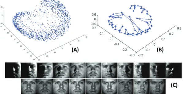
One of the leading multilinear analysis approaches is Multilinear Principal Component Analysis (MPCA), or Tensorfaces [108, 110]. This method was based on multilinear alge-bra to present relationships among factors of given data. Figure 1.3 shows an example of multifactor representation on the Extended Yale-B database. There are three subjects, each with nine poses and 64 lighting conditions chosen in this example. Figure (A) presents the distribution of the first two principal components. Meanwhile figure (B) shows the dis-tribution of 64 lighting conditions of the first subject. Finally, figure (C) shows the facial images of the first subject across 11 lighting conditions and nine different poses.

The heart of Multilinear Principal Component Analysis is to use Principal Component Analysis (PCA) [105] and Higher-order Singular Value Decomposition (HOSVD) [62] in order to decompose a given tensor. Sun et al. [100] presented the High Order

Orthogo-Figure 1.3: Multi-factors in the Extended Yale-B DB: (A) Distribution of the first two prin-cipal components trained on first three subjects with nine poses and 64 lighting conditions, (B) Distribution of 64 lighting conditions of the first subject, (C) Facial images of the first subject across 11 lighting conditions and nine different poses.

(27)

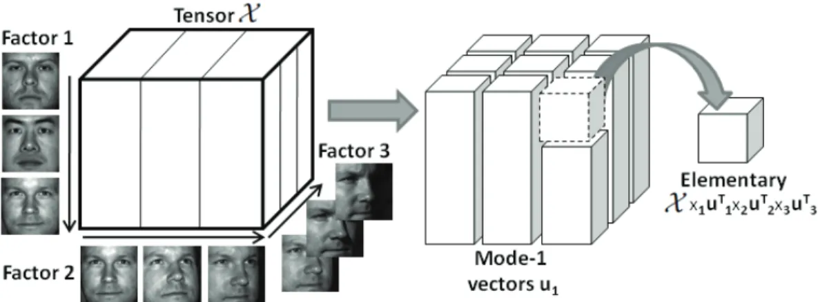
Figure 1.4: Multifactor data presented in Tensor form (left) and the corresponding elemen-tary Tensor projection (right).

nal Iteration (HOOI) to generalize the ideas of Higher-order SVD. Generalized Low Rank Approximation (GLRAM) [64, 123] proceeds the alternative projection to ﬁnd the optimal projection matrices. Recently, instead of dealing with multilinear approaches, researchers have proposed nonlinear geometrical structures created by multiple factors. Vasilescu and Terzopoulos [108, 109] presented a kernel based MPCA to analyze these nonlinear struc-tures. To ﬁt the manifold structures, created by the variations of body posture and viewpoint in the motion image space, Park and Savvides solved the multifactor analysis using mani-fold learning algorithms [79]. Pang et al. [77] presented an1-norm tensor to solve outliers

but their method can easily fail in a local minimum.

1.3

Thesis Contributions

Although widely used, Multilinear Principal Component Analysis still suffers from three major drawbacks. Firstly, it is known that MPCA cannot work on data with missing values, as shown in Figure 1.5. It is also unable to perform well on noisy data or data with outliers. Secondly, since MPCA deals with high multi-dimensional datasets, it is usually compu-tationally expensive. Therefore, it is hard to employ it in practical applications. Finally, MPCA normally loses the original local geometry structures due to the averaging process. Park and Savvides [78, 80] detailed this limitation and presented a Submanifold Preserving

(28)

Figure 1.5: (A) Tensor with missing values and (B) the tensor and multifactor ﬂattening process

Multifactor Analysis (SPMA) to keep the factor dependent geometry. The submanifold coordinate is aligned using Procrustes analysis [45] and employs the mean shape as the reference. However, their method is unable to deal with missing values and doesn’t allow for high accuracy in local alignment.

This thesis presents a novel approach named Compressed Submanifold Multifactor Analysis (CSMA) to solve the three mentioned problems. Firstly, instead of using the traditional Singular Value Decomposition (SVD), which is unable to deal with input data containing missing values and outliers, a novel Singular Value Decomposition solving via

₁-norm (SVD-₁) multifactor approach is proposed to decompose factors in given tensors. Our proposed approach can therefore avoid the distortion of outliers efficiently. Secondly, Random Projections (RP) are employed to reduce the number of dimensions of input data in order to reduce the computational time. The theories behind Random Projection in ma-trix decomposition are also provided to guarantee that it is able to preserve the properties of the compressed multifactor data. Finally, in order to avoid distortions of multifactor structures, a robust local alignment approach is employed to prevent the averaging process. In addition, this thesis also proposes a novel approach named Sparse Class-dependent Feature Analysis (SCFA), to combine the advantages of sparse representation in an over-complete dictionary, with a powerful nonlinear classifier. The classifier is based on the

(29)

estimation of class-speciﬁc optimal ﬁlters, by solving an 1-norm optimization problem.

We show how this problem is solved using the Alternating Direction Method of Multipliers (ADMM) and also explore relevant convergence details. Our method as well as its Repro-ducing Kernel Hilbert Space (RKHS) version is tolerant to the presence of noise and other variations in the image. This method achieves very high classiﬁcation accuracies when applied to the problems of face recognition and object classiﬁcation.

1.4

Thesis Organization

In chapter 1, we present the motivation for our work, a brief introduction of multiple factor analysis, and our main contributions in this thesis. The remainder of this thesis is organized as follows. Chapter 2 provides background and reviews previous multifactor analysis and tensor methods. In chapter 3, we revisit the area of Compressed Sensing, one of the hot topics in applied mathematics and computer sciences nowadays. The null-space condition, uniqueness and restricted isometry property (RIP) are discussed in detail. In addition, the

_p-norm minimization theories that are of great importance to this thesis are also reviewed carefully. In chapter 4, we present our novel Compressed Submanifold Multifactor Anal-ysis approach that is able to deal with multifactor datasets containing noisy and missing values. Our approach allows the representation of data in a compressed form, while still preserving data structures. We present our SVD-1 multifactor decomposition approach

to deal with multifactor datasets that contain missing data and outliers. The method bor-rowed from recent state-of-the-art ideas in 1-norm formulation is then solved by using

Alternative Direction Method of Multipliers optimization method. In chapter 5, we present our novel pattern classiﬁcation approach, named Sparse Class-dependent Feature Analysis, to combine the advantages of sparse representation in an overcomplete dictionary, with a powerful nonlinear classiﬁer. In order to evaluate our proposed methods, a number of ex-periments are conducted and are described in detail in chapter 6. In these exex-periments, our

(30)

methods show improvement in both efﬁciency in dealing with missing data as well as in classiﬁcation results. Finally, we provide some conclusions and scope for future work in chapter 7.

1.5

Notation

In this thesis, boldface lowercase letters represent vectors, e.g. x, and boldface uppercase letters denote matrices, e.g. X. Higher-order tensors or multidimensional data are denoted by calligraphic uppercase letters, e.g. X. Given a matrix X, X is the transpose of X. Meanwhile, ₂ denotes the ₂-norm of a vector, i.e. ∀x ∈ Rn_,_x

2 = (n_i=1x2i)1/2, 1

denotes the₁-norm of a vector, i.e. ∀x∈Rn_,_x

1 =n_i=1|xi|. In a number of studies, it

is shown that1 norm gives much sparser solution than2 norm [30, 35]. The trace-norm

of a given matrixX, denoted byX_∗, is computed by the sum of the singular values ofX. Finally,<X,Y>denotes the trace ofXY.

(31)

(32)

Chapter 2

Literature Review

One of the first studies related to tensors and multifactor analysis was carried out by Hitch-cock in 1927 [52]. In his work, a tensor was presented as a combination of a specific number ofrank-onetensors. Cattell [23] proposed new concepts to analyze multiple axes and parallel proportional representations in 1944. Based on these concepts, Carroll et al. [22] developed a method named Canonical Decomposition (CANDECOMP) in 1970 that was widely used among the researchers in the community of psychometrics in 1970. Dur-ing this period, another popular method for tensor decomposition, named PARAFAC [48], was also introduced by Harshman. CANDECOMP and PARAFAC are the state-of-the-art tensor decomposition methods that have been applied successfully in numerous areas, es-pecially in the field of brain imaging where they were called the topographic components model [48]. In 1963, another well-known method, Tucker decomposition, was introduced [103]. During its development, the method has been called by many different names, such as three-mode PCA [60], N-mode PCA [56], Higher-order SVD [62], N-mode SVD [110] and three-mode factor analysis [103]. This method has been applied successfully in a num-ber of fields, i.e. computer vision, data mining, graph analysis, signal processing, numerical analysis, numerical linear algebra, neuroscience and especially psychometrics and chemo-metrics [58, 67]. While PARAFAC and the Tucker decomposition methods are fruitful

(33)

for certain dense and structured tensors, they are still limited when applied to large-scale and sparse tensors. Hence, Savas and Elden presented Krylov-type methods for tensor decomposition and low-rank approximations in large-scale and sparse data [92]. Several Krylov-type procedures have been subsequently introduced that generalize matrix Krylov methods for tensor computations. The words “multifactor” and “tensor” are used inter-changeably with the same meaning in this thesis. A detailed review of tensor methods can be found in [58, 67].

The rest of this chapter is organized as follows. First, we review the preliminaries of multifactor analysis and higher-order tensor decompositions. We then review two main fundamental tensor decomposition methods, i.e. PARAFAC and Tucker decomposition before showing the limitations of these fundamental tensor decomposition methods.

2.1

Mutifactor Analysis Preliminaries

A tensor or a multifactor model can be represented as a multi-dimensional orN-way array, i.e. X ∈Rn1×n2×...×nN_{. In other words, as deﬁned in [58], an}_N_{th-order tensor is a result}

of the tensor product of N vector spaces deﬁned in their own coordinate system. Figure 2.1 shows an example of athird-ordertensor (N = 3). Noticeably, whenN >3, the visual representation of that higher-order tensor will become more complicated. Decompositions

(34)

Figure 2.2: Examples of tensor ﬁbers and tensor slices: (A) Mode-1 tensor ﬁbersx:,j,k, (B)

Mode-2 tensor ﬁbersx_i,_:_,k, (C) Horizontal slicesX_i,:,:

of higher-order tensors have become one of the interesting topics among applied mathe-maticians for decades [3]. Compared to matrices, higher-order tensors have a couple of differences and are more complicated in deﬁnition and representation. In this section, we review the preliminaries of tensors and provide details on the associated notation used in this thesis.

2.1.1

Tensor Terminologies

Tensor Modes

The modes of a given tensorX ∈Rn1×n2×...×nN _{are the number of different dimensions}_N

of that tensor. They are also called “orders” or “ways” in a number of published articles. Using this definition, matrices can be simply considered as tensors with a mode of two. Higher-order tensors, i.e. third-order or higher, are denoted by boldface Euler script letters as defined in section 1.5. The element(i1, i2, i3) of a third-order tensor X is denoted by x_i₁_,i₂_,i₃. Figure 2.1 shows an example of a tensor with a mode of three (N = 3). Most of tensors defined in this thesis are denoted in a restricted sense, i.e. a three-dimensional array of real values, X ∈ Rn1×n2×n3_{, where the vector space is equipped with some algebraic}

(35)

Tensor Fibers

Given anNth-order tensorX ∈Rn1×n2×...×nN_{, its tensor ﬁbers can be computed by}

keep-ing its all tensor indices except one, i.e. X:,i2,i3,...,iN, Xi1,:,i3,...,iN, ..., Xi1,i2,...,iN−1,:.Figures

2.2 (A) and (B) show two examples of mode-1 and mode-2 tensor ﬁbers of a third-order tensor. When computed from a given tensor, ﬁbers are always considered as column vec-tors.

Tensor Slices

Tensor slices have almost similar properties as tensor ﬁbers except that they involve releas-ing two factors instead of one. Given anN-order tensorX ∈ Rn1×n2×...×nN_{, its tensor slices}

can be computed by keeping its all tensor indices except two, i.e. X:,:,i3,...,iN, Xi1,:,:,i4,...,iN,

...,Xi1,i2,...,iN−2,:,:. Figure 2.2 (C) shows the horizontal tensor slides of a third-order tensor

X, denoted byX_i₁_,:,:. Alternatively, thei3-th frontal slice of a third-order tensor,X:,:,i3, may

be denoted more compactly asX_i₃.

2.1.2

Tensor Inner Product and Tensor Norm

Tensor Inner Product

Given two higher-order tensorsXandYwith the same dimensions, i.e.X,Y ∈Rn1×n2×...×nN_,

thetensor inner productis computed as in Eqn. (2.1).

X,Y = n1 i1 n2 i2 ... nN iN x_i₁_,i₂_,...,iNy_i₁_,i₂_,...,iN (2.1)

(36)

Tensor Norm

Based on the deﬁnition of tensor inner product, thetensor normor theFrobenius normof a tensorX ∈Rn1×n2×...×nN _{is simply deﬁned as in Eqn. (2.2).}

X F =X,X 1/2 = ( n1 i1 n2 i2 ... nN iN x_i₁_,i₂_,...,iNx_i₁_,i₂_,...,iN)1/2 (2.2)

Similar to the property in matrices, multilinear multiplication by orthogonal matrices does not change the Euclidean length of the corresponding ﬁbres of the tensor. Therefore, the tensor norm is invariant to any orthogonal transformation. For example, given a set of orthogonal matrices, i.e. U1,U2,U3,V1,V2, andV3, the following property in tensors has

been proven:

X F =(U1,U2,U3).X F =X.(V1,V2,V3)F (2.3)

2.1.3

Rank-One Tensor

Given anNth-order tensorX ∈Rn1×n2×...×nN_{, it is called}_rank-one_{tensor if and only if it}

can be represented as the outer product ofN vectors as in Eqn. (2.4).

X v(1)◦v(2)◦v(3) (2.4)

where “◦”denotes the outer product of vectors. In other words, each element of the tensor

X is the product of the corresponding vector elements, as deﬁned below:

x_i₁_,i₂_,...,iN v(1)_i₁ v(2)_i₂ ...v(_iN)

N ,∀ik ∈[1, nk] (2.5)

(37)

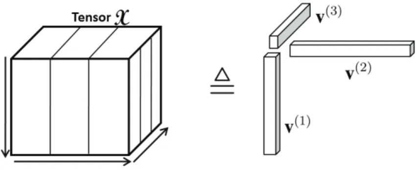
Figure 2.3: An example of tensor representation: the third-order tensor X is presented under the outer product of three vectorsv(1),v(2)andv(3).

2.1.4

Tensor Rank

Given an Nth-order tensorX ∈ Rn1×n2×...×nN_{, its} _rank_{, denoted by} _rank₍_X₎_{, is deﬁned}

as the smallest number of rank-one tensors whose sum can generate the tensor X. Rank computation in tensors are much more complicated than the one in matrices. Given a random tensor, there is no straightforward method to determine the rank of that tensor since it is an NP-hard problem [49]. In practice, in order to determine the rank of a given tensor, it is usual to numerically ﬁt various rank-Kcomponents, as is done in the PARAFAC method, discussed in section 2.2.

2.1.5

Tensor Flattening

Given an Nth-order tensor X ∈ Rn1×n2×...×nN_{, its ﬂattening, also called tensor}

unfold-ing or tensor matricization, is a technique to reorder the elements of itsNth-order tensor into a matrix. It is clear that the tensorX can be flattened along its different modes. De-tails on tensor flattening methods can be found in Kolda et al. [58]. In our work, we are only interested in mode-n flattening. The mode-n flattening of an Nth-order tensor

X ∈ Rn1×n2×...×nN _{is denoted by}_X

(n) that arranges the mode-n ﬁbers to be the columns

of the resulting matrix. Figure 2.4 shows an example of how a 2×3×2 tensor can be ﬂattened into three mode-3unfolding matrices, i.e.X(1),X(2) andX(3).

(38)

Figure 2.4: An example of tensor ﬂattening. Given a third-order tensorX ∈ R2×3×2, it can be ﬂattened in mode-3into three unfolding matricesX(1) ∈R2×3×2,X(2), andX(3).

2.1.6

n

-Mode Product

Then-mode matrix product denotes the multiplication of a tensor by a matrix or a vector in moden. Given anNth-order tensorX ∈Rn1×n2×...×nN _{and a matrix}_Y_∈ _Rm×nk_{, their} k-mode product, which is denoted by(X ×_kY), can be computed as follows:

(X ×_kY)_i₁_,i₂_,...,ik₋₁_,j,ik₊₁_,...,iN =

nk ik=1

x_i₁_,i₂_,...,iNy_j,ik (2.6)

It is to be noted that in our work, we only consider the multiplication of a tensor by a matrix. However, tensors can be also multiplied together. In that case, their notation and computation will be more complicated. [58] provides details on tensor multiplication.

2.1.7

Matrix Kronecker, Khatri-Rao and Hadamard Products

In this section, we review several important types of products, including the Kronecker product, the Khatri-Rao product, and the Hadamard product. These matrix product methods are used widely in our thesis.

(39)

Kronecker Product

Given two matricesX∈Rm1×n1_and_Y∈Rm2×n2_{, their}_{Kronecker product}_K∈R(m1m2)×(n1n2)_,

which is denoted byX⊗Y, can be computed as follows:

K=X⊗Y= ⎛ ⎜ ⎜ ⎜ ⎜ ⎜ ⎜ ⎜ ⎝ x1,1Y x1,2Y ... x1,n1Y x2,1Y x2,2Y ... x2,n1Y ... ... ... ... x_m₁_,1Y xm1,2Y ... xm1,n1Y ⎞ ⎟ ⎟ ⎟ ⎟ ⎟ ⎟ ⎟ ⎠ (m1m2)×(n1n2) (2.7) Khatri-Rao Product

Given two matricesX∈Rm1×n_and_Y_∈_Rm2×n_{, their}_{Khatri-Rao product}_R_∈_R(m1m2)×n_,

which is denoted byX Y, can be computed as follows:

R=X Y= [x1 ⊗y1,x2⊗y2, ...,xn⊗yn] (2.8)

where x_i and y_i are columns of X and Y respectively. In other words, the Khatri-Rao product can be considered as the Kronecker product of the matching columns ofXandY. Whenxandyare vectors, the Kronecker and Khatri-Rao products are identical.

Hadamard Product

Given two matrices X and Y ∈ Rm×n, their Hadamard product H ∈ Rm×n, which is denoted byX∗Y, can be computed as follows:

H=X∗Y= ⎛ ⎜ ⎜ ⎜ ⎜ ⎜ ⎜ ⎜ ⎝ x1,1y1,1 x1,2y1,2 ... x1,ny1,n x2,1y2,1 x2,2y2,2 ... x2,ny2,n ... ... ... ... x_m,₁y_m,₁ x_m,₂y_m,₂ ... x_m,ny_m,n ⎞ ⎟ ⎟ ⎟ ⎟ ⎟ ⎟ ⎟ ⎠ m×n (2.9)

(40)

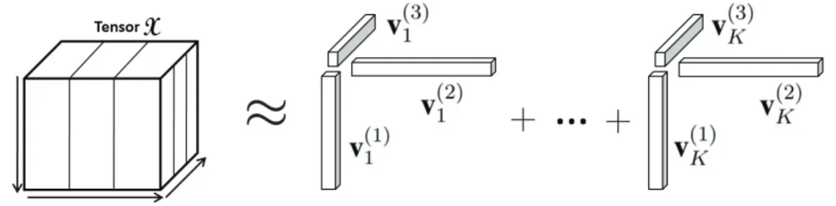
Figure 2.5: An example of PARAFAC tensor decomposition, a tensorX is approximated by a sum ofKcomponents of rank-one tensors.

2.2

PARAFAC Decomposition

The PARAFAC decomposition method factorizes a tensor into a sum of component rank-one tensors. Given a third-order tensorX ∈ Rn1×n2×n3 _{and a redeﬁned positive integer}_K_,

the PARAFAC decomposition can be calculated as follows:

X K r=1 x(1)_r ◦x(2)_r ◦x(3)_r (2.10) wherex(1)_r ∈Rn1_,_x(2)

r ∈Rn2 andxr(3) ∈Rn3, r= 1, ..., K. When denoted in element-wise

form, Eqn. (2.10) can be rewritten as follows:

x_i,j,k K

r=1

x(1)_i,rx(2)_j,rx(3)_k,r,∀i= 1, ..., n1;j = 1, ..., n2;k = 1, ..., n3. (2.11)

Generally, the PARAFAC decomposition of an Nth-order tensor X can be simply found using the Alternative Least Square (ALS) method as follows:

min

X X −

X (2.12)

whereXis calculated as given in Eqn. (2.10):

X = K r=1 λ_rx(1)_r ◦...◦x(_rN) = [λ;X(1),X(2), ...,X(N)] (2.13)

(41)

Algorithm 1PARAFAC Decomposition Method [58]

Input:TensorX, numberK Output:λ,X(i),∀i= 1, ..., N InitializeX(i) ∈Rni×K,∀i= 1, ..., N repeat for∀n∈[1..N]do V←X(1)X(1)∗...∗X(n−1)X(n−1)∗X(n+1)X(n+1)∗...∗X(N)X(N) X(n)←A(n)(X(N) ... X(n+1) X(n−1) ... X(1))V†

normalize columns ofX(n), norms are named asλ end for

untilﬁt ceases to improve or maximum iterations exhausted

In order to find X(k), the Alternative Least Square approach fixes all X(i),∀i = k. The procedure is repeated until some convergence criterion is satisfied. Assuming we want to solve forX(1), then the minimization problem can be defined as follows,

min X(1) X(1)−X (1) (X(N) X(N−1) ... X(2))_F (2.14)

whereX(1) =X(1).diag(λ). Then, we can ﬁnd the optimal solution to the problem (2.14) as follows:

X(1) =X(1)[(X(N) X(N−1) ... X(2))]† (2.15)

Due to the pseudoinverse property of the Khatri-Rao product, Eqn. (2.15) can be written as follows:

X(1) =X(1)(X(N) ... X(2))(X(N)X(N)∗...∗X(2)X(2))† (2.16)

Algorithm (1) shows the pseudocode of the PARAFAC decomposition algorithm. This method is simple to understand and implement. However, it is easy to see that there are two limitations to this method. Firstly, it is assumed that the number of component rank-one tensorsKhas to be given. Secondly, The solution is not guaranteed to converge to a global minimum. In addition, the ﬁnal solution is also heavily dependent on the starting guess. Figure 2.5 shows an example of how the FARAFAC tensor decomposition method works.

(42)

Figure 2.6: An example of Tucker decomposition, a tensorX ∈Rn1×n2×n3 _{is approximated}

by a combination of a core tensor Z ∈ Rm1×m2×m3 _{and three factor matrices, i.e.} _V₁ ∈ Rn1×m1_,_V₂ ∈Rn2×m2 _and_V₃ ∈Rn3×m3_.

Algorithm 2HOSVD Decomposition Method [58, 62]

Input:TensorX

Output:Z,X(i),∀i= 1, ..., N for∀n ∈[1..N]do

X(n) ←R_nleading left singular vectors ofX(n) end for

Z ← X ×1X(1)×2 X(2)...×N X(N),

2.3

Tucker Decomposition

Given anNth-order tensorX ∈Rn1×n2×...×nN_{, the Tucker decomposition factorizes it into}

a core tensorZ ∈ Rm1×m2×...×mN _{multiplied by a matrix}_V

i ∈Rni×mi along each modei.

Mathematically, the Tucker decomposition can be represented as follows:

X =Z ×1V1×2V2×3...×N VN =

n1,...,nN i1,...,iN

z_i₁_,...,iNV1,i1,...,iN ◦...◦VN,i1,...,iN (2.17)

Notice that these factor matrices are usually orthogonal. The Tucker decomposition became more popular after the publication of the Higher-order SVD method, that was pro-posed by Lathauwer [62]. The HOSVD decomposition method is summarized by Algo-rithm (2).

(43)

Figure 2.7: An example to show the decomposition process of the classical Singular Value Decomposition method. Given a matrixAof sized×n, the SVD method will decompose

Ainto two orthonormal matricesUandV, and a diagonal matrixΣ.

2.4

Higher-order SVD (HOSVD)

Multilinear PCA is an extension of Principal Component Analysis to multi-factor frame-works, where SVD is at the heart of the decomposition process. This section ﬁrst reviews the traditional computation of SVD and then discusses its limitations.

2.4.1

Singular Value Decomposition (SVD)

Givenn training images, each withd pixels, denoted by a 2D matrixX ∈ Rd×n_{, a pair of} singular vectorsu∈Rd_and_v_∈_Rn_of_X_{can be computed using Eqn. (2.18).}

Xv=λu and uX=λv (2.18)

whereλ ∈ Ris the correspondingsingular value. Generally,Xcan be reformulated [55] as shown below: X= r i=1 λ_iu_iv_i or X=UΣV (2.19)

whererdenotes the rank ofX, r ≤ min(d, n)andu_i ∈Rd_and_v

i ∈ Rnare orthonormal,

where each has the length of 1 and every pair is orthogonal, i.e.UU=IandVV=I.Σ is a diagonal matrix containing the square root of the eigenvalues ofUorVin descending order. Each (u_i,v_i) pair forms a pair of left and right singular vectors with singular value

λ_i > 0, whereλ_k ≥ λ_k+1,∀k ∈ [1, r− 1]. It follows that each ui is an eigenvector of XX and eachv_i is an eigenvector ofXX, and the corresponding eigenvalues areλ2_i. In

(44)

Figure 2.8: An example to show the decomposition process of the Higher-order SVD method. Given a third-order tensorX, HOSVD method will decompose it into three matri-cesV1,V2 andV3, the core tensorZ and the matrixUthat satisfy the HOSVD condition.

order to ﬁnd the top singular vectors, the unit vectorv1 that maximizesXvwill be ﬁrst

computed and then u1 is found from that. Generally, to compute the complete SVD, we

ﬁrst ﬁnd u1,v1 and λ1. Then we iteratively employ this on the matrix (X−λ1u1v1). In

other words, a rank-1 matrix is subtracted at each iteration.

2.4.2

Higher-Order SVD (HOSVD)

Higher-Order SVD [62] is a multilinear generalization of Singular Value Decomposition. Given an Nth-order tensor X, HOSVD can decompose it into a core tensor Z and N

orthogonal matrices, i.e. a matrix U for pixel values and N matrices V_i to represent N

factors. Without lost of generality, assume thatn = 3. Thus, a tensorX ∈ Rd×n1×n2×n3

can be decomposed using HOSVD as follows:

X =Z ×1 U×2V1 ×3V2 ×4V3 (2.20)

where×_kis thek-modematrix product of a tensor, as deﬁned in Section 2.1.6. Figure 2.9 (top) shows an example of the HOSVD decomposition. In Multilinear PCA, HOSVD is

(45)

Figure 2.9: Higher-order SVD is a multilinear generalization of the SVD. In HOSVD, the third-order tensorX is decomposed into one core tensorZ and three orthogonal matrices: matrixU(pixels), factor V1 (subjects), and factor V2 (lighting). The columns of each

or-thogonal matrix form the basis of each of the three vector spaces of a tensorX. In MPCA, HOSVD is reformulated in terms of matrices, instead of tensors, using the Kronecker prod-uct. In MPCA, the ﬁrst three images of subject 1 are represented on the ﬁrst columnV1₁ of

V₁, while the next three images of subject 2 depend on the second columnV2₁ ofV₁. The same representation is used for 3 lighting conditions V₂. Note that U is identical to the matrixUin PCA.

reformulated in terms of matrices, instead of tensors, using the Kronecker product. The equivalent form of Eqn. (2.20) in MPCA can be presented as follows,

X=UZ(V1⊗V2⊗V3) (2.21)

where ⊗ denotes the Kronecker product (defined in section 2.1.7). U is identical to the matrixUin Eqn. (2.19). A matrixZresults from the pixel-mode flattening of a core tensor presented in [108]. V_kis the right singular vector matrix of the flatten tensor Xalong the factork. From Eqn. (2.21),Zcan be derived as follows,

Z=UX(V1⊗V2⊗V3) (2.22)

(46)

Chapter 3

Compressed Sensing Revisited

3.1

Sensing Method

The revolutionary fields of compressed sensing and sparse signal approximation have been rapidly developed during this decade [6, 16, 18, 19, 20, 21, 29, 87]. Alongside the ac-celerated growth in numerous applications, such as: medical image processing [68, 69], single-pixel imaging [32], face recognition systems [113, 114], etc., the theories of sparse and compressible signal representation have been fully enriched by many researchers in this field [16, 19, 87]. Compressed sensing [88, 101] is defined as a signal acquisition paradigm that allows recovering estimates of compressible and sparse signals from high ambient dimensions N using linear measurements M with much fewer dimensions (i.e.,

M N). Therefore, the protocol in compressed sensing aims to directly acquire only important information from a given signal. This approach has the ability to acquire and recover signals in the most efﬁcient way possible and avoid a data deluge.

3.1.1

Motivation

The motivation for compressed sensing can be envisioned by considering the following problem. Given a matrixΦof size M ×N, where M N, and a signal y ∈ RM_{, the}

(47)

question that arises is if there exists asparsevector xsuch that y Φx or not. In other words, we want to ﬁnd a sparse vector or a set of sparse coefﬁcientsxso that the signaly

can be approximated by projecting this sparse vectorx onto the given dictionaryΦ. The sparsity in this case is measured by counting the number of non-zero entries in a given vector, i.e.,x₀ = number of non-zero entries inx0 = _iI(xi = 0). It is clear that the

number of non-zero entries inxhas to be smaller or equal toM at most. The matrixΦis also called a dictionary or overcomplete dictionary or frame in some contexts. From these definitions, the problem can be redefined as a problem of finding the sparsest vectorx0that

satisﬁes the linear system y = Φx. In the optimization framework, the problem can be denoted as shown in Eqn. (3.1).

P(0) : min

x x0 subject to y=Φx (3.1)

There are three important questions regarding Eqn. 3.1 that need to be answered that have resulted in three key research topics in compressed sensing [90]. Firstly, when is the solu-tion toP(0), as shown in Eqn. (3.1), unique? Secondly, what are the most efﬁcient ways to solve forP(0)? Finally, given a training data setX =x1,x2, ...,xN, how can we learn a

dictionaryΦso that it can support sparse representations on the training data setX?

There are many variants ofP(0) in the deﬁnition of the Eqn. (3.1). They are listed in the following equations:

min x x0 subject to y=Φx (3.2a) min x x0 subject to y−Φx ≤ (3.2b) min x y−Φx subject to x0 ≤K (3.2c) min x y−Φx 2₊_τ2_x 0 (3.2d)

(48)

number of non-zero entries allowed in reconstructed signals, τ is a trade-off parameter between sparsity and reconstruction ﬁdelity. It must be noted that if the support set Ω

is given in the solution to P(0), then the problem reduces to that of a simple feasibility problem, i.e. y ∈ R(ΦΩ), as in numerous well-known problems such Matching Pursuit

(MP) [11, 74], Orthogonal Matching Pursuit (OMP) [83], etc. However, it is very hard to ﬁnd the support setΩin practical applications. One approach is to enumerate all possible supports, and then pick the the smallest one that leads to a feasible solution. This method, however, is a combinatorial and exponential time algorithm, sinceP(0)is reducible to an NP-complete problem. In a general case, this problem cannot be solved in polynomial time. However, a fast solution may exist in some special cases of signals. In this section, we discuss when signals can be recovered.

3.1.2

Null-space Condition

Given a matrixΦ∈RM×N, thenull-spaceof the matrixΦis deﬁned as follows:

N(Φ) = α:Φα =0. (3.3)

From this deﬁnition, it can be concluded that for any two distinct sparse signals x and

x that need to be recovered, where x,x ∈ Σ_k, the following constraint holds: x = x. This is because it is impossible to ﬁnd two different vectorsxandx from the same given measurementyand the same dictionary Φas in Eqn. (3.1) with the constraint ofx = x. Assume thatΦx=Φx. Then we haveΦx−Φx =0orΦ(x−x) =0, where(x−x)∈Σ_k. From this condition, the signalxcan be uniquely recovered from dictionaryΦif and only if there doesn’t exist any vector in Σ₂_k in the null-spaceN(Φ). In compressed sensing, thesparkproperty is one of the most common method used to evaluate this condition. The spark computation will be discussed in detail in section 3.1.3. The fundamental idea in this section is that sparse vectors in the null-space of the matrix have to limit uniqueness. Such

(49)

conditions are referred to as null-space conditions.

Given a matrix Φ ∈ RM×N_{, assume that these exists a vector} _η _∈ _N₍_Φ₎ _{such that}

η₀ ≤ 2K. LetΩbe the support set,Ω = supp(η). Now, we can construct aK-sparse vectorx, such thatsupp(x) = Λ⊂Ω, andxΛ =ηΛ. Giveny=Φx, bothxand(x−η)are

in the solution set, furthermorex−η₀ ≤ x₀.

3.1.3

Spark

Deﬁnition of Spark [35]. The spark of a matrixΦ= [φ₁,φ₂, ...,φ_N],φ_i ∈RM _{is deﬁned} as thesmallestset of linearlydependentcolumns.

The definition ofSpark(Φ)is contrast to the one ofRank(Φ)defined as the largest set of linearly independent columns. From the spark definition, the following condition can be deduced:

2≤Spark(Φ)≤Rank(Φ) + 1 =M + 1 (3.4)

In practice, dictionaries are typically full-rank and overcomplete, withM < N. Matrices whose entries are independent and identically distributed (i.i.d.) sampled from random distributions typically haveSpark(Φ) =M + 1. Given a random square matrixΦof size

M ×M, such as Gaussian ones, it is almost surely non-singular.

Lemma (Null-space and Spark Constraint) [35]. Ifn∈N(Φ), then

n0 ≥Spark(Φ)

Proof. Assume that∃n∈N(Φ), and we haven₀ < Spark(Φ). Then, letΩ =supp(n) =i|n_i = 0.

It is to be noted that|Ω|=n₀ < Spark(Φ).

(50)

Hence, Spark(Φ) ≤ |Ω| =n₀ < Spark(Φ). This is a contradiction and therefore the lemma is true.

3.1.4

Uniqueness via Spark

Theorem (Gorodnitsky-Rao, 1997; Donoho-Elad, 2003). If a system y = Φx has a solutionx0 such thatx0 < Spark(Φ)/2, thenx0 is also the unique sparsest solution.

Proof. Recall from Lemma of null-space and spark constraint, that Ifn∈N(Φ)thenn₀ ≥Spark(Φ).

Suppose∃x0,z0 such thaty=Φx0 =Φz0 andz00 <x00.

Then, sinceΦ(z0−x0) = 0, therefore(z0−x0)is also in null-space, i.e. (z0−x0)∈

N(Φ). From the deﬁnition of spark, we have:

x00 +z00 ≥ x0+z00 ≥spark(Φ).

This result contradicts clearly the theorem above, wherex₀ < Spark(Φ)/2. Therefore,

x0 is the unique sparsest solution.

However, spark usually cannot be computed in practice. It is immediately clear that there areC_SN subset selections needed to be veriﬁed eitherSpark(Φ)≤SorSpark(Φ)≥

S. The computation of Spark(Φ) is a combinatorial problem. Its computation is quite expensive. Therefore, we resort tocoherenceas a way to estimate, at least the lower bound, the spark.

3.1.5

Coherence

Deﬁnition of Coherence [35]. Given a matrixΦ= [φ₁,φ₂, ...,φ_N]with unit-norm columns

(φ_j= 1), itsmutual coherenceis deﬁned as the largest absolute normalized inner prod-uct between different columns in Φ. Generally, the mutual coherence μ(Φ)is denoted as

(51)

follows:

μ(Φ) = max

1≤i,j≤N,i=j

|φ_i,φ_j|

φ_i.φ_j

The mutual-coherenceμ(Φ)measures how similar two elements of the given dictionary

Φ. In other words, it is a way to evaluate the dependence between columns inΦ. When the dictionaryΦis unitary where all pairwise columns are orthogonal, then mutual-coherence

μ(Φ) equals zero. In the regular cases of compressed sensing, where the dictionary Φ usually has more columns than rows, the mutual-coherence μ(Φ) must be positive. In addition, the smaller mutual-coherenceμ(Φ)is, the better it is to support representations with higher sparsity. Ideally, we always aim to achieve the smallest possible coherence in a given very large dictionary. However, it is usually impossible in practice. The following theorem shows the lower bound of the coherenceμcomputed from a dictionaryΦ.

Theorem (Welsh, 1974; Strohmer-Heath, 2004). Given a generalM ×N full-rank dic-tionaryΦ, where(M N), the following condition always holds:

μ(Φ)≥ N −M M(N −1) ≈ 1 √ M

Proof. This theorem can be proved as follows:

LetG=ΦΦ, then it is clear thatRank(G) =M, Letλ_i be the eigenvalues ofG, wherei= 1, ..., M.

Then, we have M_i₌₁λ_i = T race(G) = N. Apply 2 − 1 norm equivalence, the

following condition is achieved:

G2_F =

i

λ2_i ≥