https://doi.org/10.5194/gmd-12-3419-2019 © Author(s) 2019. This work is distributed under the Creative Commons Attribution 4.0 License.
Climate projections of a multivariate heat stress index: the role of
downscaling and bias correction
Ana Casanueva1,a, Sven Kotlarski1, Sixto Herrera2, Andreas M. Fischer1, Tord Kjellstrom3,4, and Cornelia Schwierz1 1Federal Office of Meteorology and Climatology MeteoSwiss, Zurich, Switzerland
2Meteorology Group, Dept. Applied Mathematics and Computer Sciences, University of Cantabria, Santander, Spain 3Centre for Technological Research and Innovation (CETRI), Limmasol, Cyprus
4National Center for Epidemiology and Population Health, Australian National University, Canberra, Australia acurrently at: Meteorology Group, Dept. Applied Mathematics and Computer Sciences,
University of Cantabria, Santander, Spain
Correspondence:Ana Casanueva ([email protected]) Received: 20 November 2018 – Discussion started: 14 January 2019 Revised: 11 July 2019 – Accepted: 15 July 2019 – Published: 5 August 2019
Abstract.Along with the higher demand for bias-corrected data for climate impact studies, the number of available data sets has largely increased in recent years. For instance, the Inter-Sectoral Impact Model Intercomparison Project (ISIMIP) constitutes a framework for consistently project-ing the impacts of climate change across affected sectors and spatial scales. These data are very attractive for any impact application since they offer worldwide bias-corrected data based on global climate models (GCMs). In a complemen-tary way, the CORDEX initiative has incorporated experi-ments based on regionally downscaled bias-corrected data by means of debiasing and quantile mapping (QM) methods. In light of this situation, it is challenging to distil the most ac-curate and useful information for climate services, but at the same time it creates a perfect framework for intercomparison and sensitivity analyses.
In the present study, the trend-preserving ISIMIP method and empirical QM are applied to climate model simula-tions that were carried out at different spatial resolusimula-tions (CMIP5 GCM and EURO-CORDEX regional climate mod-els (RCMs), at approximately 150, 50 and 12 km horizontal resolution) in order to assess the role of downscaling and bias correction in a multivariate framework. The analysis is car-ried out for the wet-bulb globe temperature (WBGT), a heat stress index that is commonly used in the context of work-ing people and labour productivity. WBGT for shaded condi-tions depends on air temperature and dew-point temperature, which in this work are individually bias corrected prior to
the index calculation. Our results show that the added value of RCMs with respect to the driving GCM is limited after bias correction. The two bias correction methods are able to adjust the central part of the WBGT distribution, but some added value of QM is found in WBGT percentiles and in the inter-variable relationships. The evaluation in present climate of such multivariate indices should be performed with cau-tion since biases in the individual variables might compen-sate, thus leading to better performance for the wrong rea-son. Climate change projections of WBGT reveal a larger in-crease in summer mean heat stress for the GCM than for the RCMs, related to the well-known reduced summer warming of the EURO-CORDEX RCMs. These differences are low-ered after QM, since this bias correction method modifies the change signals and brings the results for the GCM and RCMs closer to each other. We also highlight the need for large ensembles of simulations to assess the feasibility of the derived projections.
1 Introduction
Jones et al., 2011; CORDEX-Adjust). Due to this, there have been many efforts towards the distillation of climate data into usable climate information (Hewitson et al., 2014; Fernán-dez et al., 2018). This is largely hampered by the large enve-lope of uncertainty, which grows in the subsequent steps in the production of climate information, the so-called “uncer-tainty cascade” (Wilby and Dessai, 2010). In this work we assess the role of downscaling and bias correction as key el-ements in the development of climate information. For this purpose, we intercompare climate change projections of heat stress in Europe coming from different data sources, at dif-ferent spatial resolution and corrected with two difdif-ferent bias correction methods, in order to identify the major sources of uncertainty in terms of present and future climate.
Global climate models (GCMs) are able to reproduce the main features of the climate system and are commonly used to examine changes in climate on a global scale (Taylor et al., 2011). Despite recent improvements, systematic biases remain and the model resolution is still too coarse to ade-quately describe mesoscale processes (Giorgi and Mearns, 1991). Regional climate models (RCMs) are frequently used to bridge the gap between the GCM and the regional to local scales (Giorgi, 2006; Feser et al., 2011). They solve the gov-erning equations of the climate system in a limited spatial domain using initial and boundary conditions from GCMs (reanalysis for model evaluation experiments). Despite the increased horizontal resolution, RCMs, similar to GCMs, in-clude physical parameterisations for subgrid processes which occur at spatial scales smaller than the model grid spacing (microphysics, convection, radiation, etc.). RCMs add valu-able information with respect to their driving GCM due to more detailed spatial patterns and the better representation of local processes, e.g. high precipitation frequencies (see e.g. Maraun et al., 2010; Warrach-Sagi et al., 2013). However, both GCMs and RCMs are prone to systematic biases and some sort of bias adjustment or correction is typically needed before they are used in impact modelling (Christensen et al., 2008; Hagemann et al., 2011). Bias correction (BC) meth-ods typically adjust some features of the model distribution (e.g. the mean or percentiles) towards the observed counter-parts, partly removing systematic errors in the model out-put. However, the added value of bias-corrected RCM simu-lations with respect to the bias-corrected GCM counterparts remains unclear. The same question applies for the difference between bias-corrected high-resolution RCM simulations (at approximately 12 km) and the coarser counterparts (at ap-proximately 50 km). For the latter, Casanueva et al. (2016) showed that the added value (in terms of mean, percentiles and precipitation frequency) is not statistically significant af-ter applying simple (scaling) bias correction methods.
Many BC methods with different characteristics have been described in the literature (Maraun et al., 2010; Piani et al., 2010; Gutiérrez et al., 2019): empirical or parametric meth-ods, variable-specific (e.g. assuming a certain distribution) or nonspecific methods, multivariate or univariate methods, and
seamless or for specific time horizons (e.g. the correction of ensemble spread in monthly–seasonal forecasts). All of them consist of a training phase (in which the correction function is calibrated) and an application phase under different condi-tions. Note that the correction functions (calibrated in present climate) are assumed to be invariant on time (stationarity as-sumption). Moreover, in a climate change context, the way the correction is applied in future climate might affect the climate change signal.
A specific bias correction method was developed in the framework of the ISIMIP initiative (Warszawski et al., 2014). This project attempted to offer a consistent framework for cross-sectoral, cross-scale modelling of the impacts of cli-mate change in order to ease the application of clicli-mate model data and meet user-specific needs. The ISIMIP method (Hempel et al., 2013; ISIMIP2b, Frieler et al., 2017) was applied to several GCMs from CMIP5 (the Coupled Model Intercomparison Project Phase 5; Taylor et al., 2011). The ready-to-use, bias-corrected data have been used to produce impact model simulations for different sectors such as agri-culture, biomes, forests and fisheries permafrost, as well as to derive climate impact indices, including heat stress (Kjell-strom et al., 2018).
Among other BC methods, empirical quantile mapping stands out as one of the most widely used methods. Despite its limitations and shortcomings (Maraun et al., 2017; Lan-zante et al., 2018), it is one of the best-performing bias cor-rection and statistical downscaling methods in evaluation ex-periments (Gutiérrez et al., 2019; Hertig et al., 2019). One reason for this might be that it is often favoured by the eval-uation metrics – commonly based on moments of the prob-ability density function – considered in intercomparison ex-periments. Quantile mapping is, by construction, able to cor-rect for intensity-dependent biases (i.e. biases that change throughout the distribution; Gobiet et al., 2015). As a conse-quence, it can modify the raw model climate change signal, which might be debatable (Gobiet et al., 2015; Casanueva et al., 2018; Ivanov et al., 2018). In contrast, the main objective of the ISIMIP correction is to preserve the trend of the raw data in the calibration period.
In the present work, we consider CMIP5 and EURO-CORDEX (European branch of EURO-CORDEX) simulations, the latter at the two available spatial resolutions (approximately 12 and 50 km), and the ISIMIP correction and empirical quantile mapping as bias correction methods for the follow-ing purposes:
– to assess the added value of a more complex (in terms of the number of parameters calibrated) bias correction method (empirical quantile mapping) with respect to the ISIMIP correction;
– to assess the impact of downscaling and bias correction in the climate change signal.
The added value is examined by evaluating several statistics under present climate conditions and exploring the feasibil-ity of climate change projections. All analyses are applied in the context of climate change projections of heat stress in Europe. Heat stress depends mainly on temperature and humidity (low wind speed and high solar radiation also con-tribute to heat stress but are not considered in this work). Whereas empirical quantile mapping is a univariate bias cor-rection method (typically with the same core implementa-tion for all variables when it is applied in a multivariate con-text), the ISIMIP correction includes dependencies between some variables (e.g. mean temperature is needed to correct maximum–minimum temperatures) in order to preserve the physical consistency among them. Hence, the ability of the methods to reproduce multivariate structures is implicitly in-vestigated.
2 Data and methods 2.1 Heat stress index
Under very hot and humid conditions, the ability of the hu-man body to regulate the core temperature and dissipate heat via sweat evaporation is reduced, provoking heat stress (Koppe et al., 2004; Parsons, 2014). Other meteorological variables such as strong radiation or low wind speed can ex-acerbate heat stress. Such conditions directly affect human well-being and can develop into heat-related illnesses such as fatigue, muscle cramps and heat stroke. In the context of working people, several studies have revealed the neg-ative impact of heat stress on workers’ health (Pogaˇcar et al., 2018) and labour productivity (Kjellstrom et al., 2009; Ioannou et al., 2017). International organisations such as the International Standards Organization (ISO) and the US Na-tional Institute for OccupaNa-tional Safety and Health (NIOSH) have developed guidelines to protect working people against heat stress (ISO, 1989, 2017; NIOSH, 2016). The recommen-dations comprise work–rest cycles and water intake under specific heat conditions. A combination of technical, regu-latory and behavioural measures is needed to adapt work-ers to increasing temperatures at an individual, sectoral and governmental level (Vivid Economics, 2017). In the con-text of global warming, the development and dissemina-tion of heat-health planning and warning systems is now among the priorities of the World Meteorological Organi-zation (WMO) and the World Health OrganiOrgani-zation (WHO; WMO, 2015), as well as the International Labour Organiza-tion (UNDP/ILO, 2016) and the InternaOrganiza-tional OrganizaOrganiza-tion for Migration (IOM, 2016). Within this framework, the Hori-zon 2020 HEAT-SHIELD project (https://www.heat-shield. eu/, last access: 2 August 2019) aims to address the effects of climate change on the European working population within
an inter-sectoral framework (Nybo et al., 2017). In particu-lar, one of the specific objectives of the project is to generate climate change projections of heat stress (Casanueva et al., 2019).
There are many indices based on meteorological vari-ables which have been often used to assess occupational heat stress conditions in the literature (de Freitas and Grigorieva, 2015; Coccolo et al., 2016). The wet-bulb globe temperature (WBGT) has been chosen in the HEAT-SHIELD project as the primary heat stress index since it can be computed from standard meteorological variables available in both observa-tions and climate models, it can be interpreted by occupa-tional scientists and physicians by means of the correspond-ing international (ISO) and national (e.g. NIOSH, 2016) stan-dards regulations, and it can be adjusted according to the workers’ clothing.
In this study we focus on the WBGT in the shade (Bernard and Pourmoghani, 1999; Lemke and Kjellstrom, 2012), which assumes that there are no strong radiation sources (the globe temperature equals the air temperature) and wind speed of 1 m s−1, which corresponds to the movement of arms or legs during work. Bearing this in mind, the input variables for the calculation of the WBGT in the shade are air tem-perature and dew-point temtem-perature. The latter accounts for the humidity conditions and can be obtained from daily mean temperature and relative humidity (or specific humidity and air pressure) in models and observational data sets. In order to account for the highest daily heat stress, we used daily maximum temperature and daily mean dew-point tempera-ture (unlike relative humidity, it usually only slightly varies along the day) to approximate the daily maximum WBGT (Casanueva et al., 2019). WBGT is calculated through the R packageHeatStress(see the “Code availability” section). 2.2 Observational data
2.3 Global and regional climate model data
The GCM considered in the present analysis is HadGEM2-ES_r1i1p1 (Collins et al., 2011; denoted as HadGEM along the paper) from CMIP5, which is one of the GCMs used in the ISIMIP experiments. Data covering the EURO-CORDEX domain were extracted considering only land grid boxes (land area fraction larger than 50 %).
We additionally use the EURO-CORDEX RCM simula-tions (Jacob et al., 2014; Kotlarski et al., 2014) driven by HadGEM2-ES accessible via the Earth System Grid Feder-ation (ESGF archive; https://esgf.llnl.gov, last access: 2 Au-gust 2019) as of May 2017. These are the same HadGEM-driven RCM simulations as used by Casanueva et al. (2019) in a comprehensive study about climate projections of heat stress in Europe. The RCM simulations were conducted at two different spatial resolutions which correspond to approx-imately 12 (EUR-11) and 50 km (EUR-44) grid spacing. The final set of regional models consists of RACMO, CCLM and RCA run by the KNMI (Royal Netherlands Meteorological Institute), CLMcom (Climate Limited-area Modelling Com-munity) and SMHI (Swedish Meteorological and Hydrolog-ical Institute), respectively. The historHydrolog-ical simulations cover the common historical period 1981–2005 (the 5 years 2006– 2010 from the scenario simulations are added in this work to complete the observational period) and future projections cover the period up to 2099. The available RCPs (Represen-tative Concentration Pathways) vary for each GCM–RCM combination (Table 1).
We retrieved GCM and GCM–RCM data for daily max-imum temperature, as well as daily mean temperature and relative humidity (or specific humidity and sea level or sur-face air pressure, depending on the model), which were used to calculate daily mean dew-point temperature. Note that HadGEM and the HadGEM-driven RCMs present a 360 d calendar, so to harmonise this with the observations, five (or six in a leap year) missing values were included randomly along each year but keeping the same position for all vari-ables (to avoid inter-variable modifications), RCPs and mod-els. All analyses were carried out at the spatial resolution of the observational grid (regular 50×50 km). For this reason, all model simulations (GCM and GCM–RCMs) were vatively remapped into the WFDEI grid (first-order conser-vative remapping, as in the ISIMIP experiments). As a conse-quence, there will be aspects of the added value of the high-resolution EUR-11 experiments (related to better-resolved, fine-scale processes; Prein et al., 2016) that can be smoothed out, but they may still be present after remapping them onto a coarse resolution (Casanueva et al., 2016).
2.4 Bias correction methods 2.4.1 ISIMIP bias correction
The ISIMIP bias correction was developed in the framework of ISIMIP (Hempel et al., 2013). It consists of a correction of the monthly mean biases followed by the correction of the daily variability around the monthly mean. For temper-ature the monthly correction is additive, whereas it is mul-tiplicative for precipitation, radiation and wind. The daily variability correction consists of a parametric quantile map-ping adjusting a normal distribution for temperature and a gamma distribution for precipitation. After ISIMIP (see light green dashed line in Fig. 1a, b), the mean of the historical data is adjusted towards the observations (black lines), but the variance and shape of the raw distribution are mostly re-tained. The monthly means and monthly variability are ad-justed using only a constant correction (either an offset or a multiplicative factor) in the historical and future periods (see green lines in Fig. 1a, b for an example for temperature; light and dark green lines represent the historical and future bias-corrected data through ISIMIP, respectively). Therefore, the corrections cancel out when calculating the mean (additive or relative) climate change signal, and the long-term trend of the raw simulated variables (red arrow in Fig. 1b) is preserved.
The ISIMIP correction includes dependencies between some variables (e.g. mean temperature and wind speed are needed to correct maximum–minimum temperatures and eastward–northward wind components, respectively) in or-der to preserve the physical consistency among them. How-ever, there are no implemented dependencies between tem-perature and relative humidity yet. This BC method is imple-mented for several variables as part of the R package down-scaleR (Bedia et al., 2017), included in the R bundle cli-mate4R(Cofiño et al., 2018; Iturbide et al., 2019). We correct dew-point temperature following the same procedure as for daily mean temperature; thus, dependencies with other vari-ables are not considered. As mentioned before, daily mean temperature is used in the correction of the daily maximum temperature in order to maintain the physical consistency between variables. Although the ISIMIP initiative provides bias-corrected GCM data, for the sake of consistency we ap-ply the corrections to the raw GCM as well as RCM data.
2.4.2 Empirical quantile mapping (QM)
In this work we use the implementation from Déqué (2007) and Rajczak et al. (2016), included in the R package
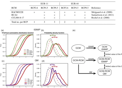
Table 1.EURO-CORDEX RCMs driven by HadGEM for two spatial resolutions (EUR-11 for approximately 12 km spatial resolution and EUR-44 for approximately 50 km resolution) and three RCPs (RCP2.6, RCP4.5 and RCP8.5).
EUR-11 EUR-44
RCM RCP2.6 RCP4.5 RCP8.5 RCP2.6 RCP4.5 RCP8.5 Reference
RACMO22E × × × × × × Meijgaard et al. (2008) RCA4 × × × × × Samuelsson et al. (2011) CCLM4-8-17 × × × Rockel et al. (2008)
Total no. per RCP 1 3 3 2 2 3
Figure 1. (a–d)Illustrative example of the effect of the two bias correction methods on the empirical cumulative distribution function(a, c)and the probability density function(b, d)for either RCM or GCM data. Observations are depicted in black and historical (HIST) and future (FUT) model simulations in light and dark colours, respectively. Raw data are depicted in red, ISIMIP-corrected data in green(a, b)and QM-corrected data in purple(c, d). The magnitude of the mean change signal is shown with the arrows. This example corresponds to daily maximum temperature as represented by HadGEM for an exemplary grid box (HIST: 1981–2010, FUT: 2070–2099 for RCP8.5). (e)Conceptual scheme of the present study.
above (below) the calibration range (Themeßl et al., 2012). The correction is calibrated for each day of the year with a 91 d moving window. It is a univariate BC method and in this work it was applied independently to daily maximum tem-perature and daily mean dew-point temtem-perature.
For a historical simulation (see e.g. light purple dashed lines in Fig. 1c, d) the corrected data largely resemble the dis-tribution of the observations. During the application of QM to a future climate simulation, the model data are mapped into the percentiles of the training data and the corresponding correction function is applied (dark purple lines in Fig. 1c, d); thus, QM would differently correct the future and the histor-ical distributions if the relative frequencies in the future dif-fer from the training counterparts (Casanueva et al., 2018).
cen-tury (2070–2099) to produce bias-corrected climate projec-tions. Due to the multivariate nature of the WBGT, we sep-arately correct daily maximum temperature and daily mean dew-point temperature prior to the WBGT calculation (i.e. the component-wise approach; Casanueva et al., 2018). Al-though the BC methods are applied to the full time series (monthly mean correction for ISIMIP, 91 d moving window centred on each day of the year for QM), all results shown refer to the summer season (June, July, August), since it is the time when extreme heat stress conditions occur.
As shown in Fig. 1e, the ISIMIP bias correction is ap-plied to the GCM and the RCMs to assess the added value of the RCMs after bias correction. We additionally correct the climate models using quantile mapping to assess the added value of a more complex (in terms of the number of parame-ters calibrated) bias correction method.
2.5 Evaluation metrics
The performance of the raw and bias-corrected data is firstly evaluated by using the mean bias (model minus observations) of several parameters of the distribution, such as the mean and 95th and 99th percentiles of the WBGT.
Pearson correlation coefficients (Pearson, 1895) between the daily series of maximum temperature and dew-point tem-perature are obtained to show the linear dependency between the two input variables in the modelled and observed data. In order to further assess the inter-variable relationships, two-dimensional kernel densities are constructed combining the distribution of the two input variables. The representation of the two-dimensional densities shows the probability of hav-ing different combinations of daily maximum and dew-point temperatures. Density plots are obtained for the raw and bias-corrected data and compared to the observation counterparts. Perkins et al. (2007) introduced a skill score which deter-mines the similarity between two probability density func-tions (PDFs). It is a very useful metric since it allows for a comparison across the entire distribution. It measures the common area between two PDFs by calculating the cumu-lative minimum value of two distributions of each binned value (skill scores of 1 mean perfect performance). Here a two-dimensional extension of the Perkins skill score is used, obtained from two-dimensional kernel densities instead of univariate PDFs. Therefore the cumulative minimum value is calculated in a two-dimensional field and the score shows the similarity (overlap) between the modelled joint distribu-tion of daily maximum and dew-point temperatures and the observed counterpart.
3 Results
3.1 Evaluation of mean biases of WGBT
The two BC methods (ISIMIP and QM) are applied to the two primary variables of the heat stress index, namely daily
maximum air temperature and daily mean dew-point tem-perature, prior to the WBGT calculation. Under no cross-validation (i.e. the methods are calibrated and validated in the same period) both BC methods adjust, by construction, the central part of the distribution (mean for ISIMIP, median for QM; see Fig. 1a–d). ISIMIP further adjusts the variabil-ity around the mean, whereas QM additionally adjusts the 99 empirical percentiles. The performance in terms of mean bi-ases of the two BC methods for individual variables is good and differences related to the parametric (ISIMIP) or empir-ical (QM) nature of the method may arise on the tails of the distribution, for which QM outperforms ISIMIP (not shown). The suitability of the component-wise BC approach of the WBGT prior to its application in a climate change context is assessed by evaluating the corrected WBGT with the ob-served counterpart for the period 1981–2010. Although the calibration and validation periods are the same, our approach can be considered independent since the evaluated aspect (i.e. multivariate consistency and WBGT statistics) is not directly tackled by the BC methods. An additional split-sample cross-validation (cold vs. warm years; not shown) indicates that WBGT biases are of the same order of magnitude as in the non-cross-validated analysis.
Mean biases of summer mean WBGT (Fig. 2a) are evi-dent for the raw GCM and RCMs (blue boxes; note that no height correction has been applied to the raw data, which might be mainly responsible for the skewed distribution of the raw biases). These are largely reduced after both BC methods, equally well for GCM and RCM data. The eval-uation of the 95th and 99th percentiles reveals better perfor-mance for ISIMIP or QM depending on the model (Fig. 2b, c). QM improves on mean biases and reduces their variabil-ity in higher percentiles for the GCM, RACMO and RCA, whereas a cold bias emerges for CCLM. There is no evident added value of the RCMs with respect to the GCM after bias correction (see also the spatial pattern of the differences be-tween bias-corrected GCM and RCMs in Fig. S1 in the Sup-plement). This is in agreement with the findings for coarser vs. the higher resolution of RCM simulations by Casanueva et al. (2016).
Figure 2.Biases of mean(a), 95th percentile(b)and 99th percentile(c)summer WBGT for the GCM and RCMs at EUR-44 and EUR-11. Biases are calculated as model minus observations. Each box represents the biases across all grid boxes for raw (blue), ISIMIP corrected (orange) and QM corrected (green). Due to the different land–sea masks in the observations, the GCM and RCMs (EUR-44 and EUR-11), all box plots consider the grid boxes common to all data sets.
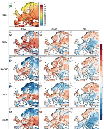
Europe (Figs. 3m and S2h). The causes for that are analysed in more detail in the next section.
3.2 Evaluation of inter-variable relationships
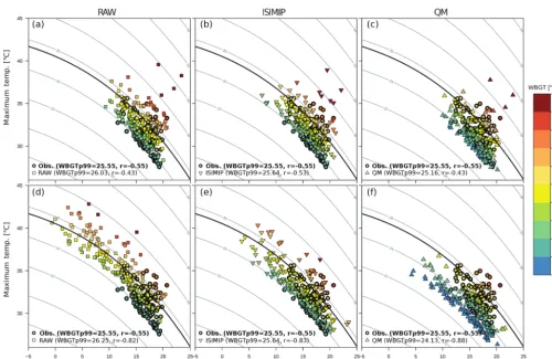
The component-wise correction of the WBGT is able to cor-rect for large biases in some WBGT statistics, but some bi-ases remain for specific locations and models. We focus on the eastern European region and select the closest grid box to the city of Warsaw (Poland), where the original positive bias of WBGTp99 (0.7◦C) turns into a negative bias (−1.4◦C)
Figure 3.Spatial distribution of the observed 99th percentile of summer WBGT (WBGTp99,a) and model biases for the GCM(b–d)and RCMs at EUR-11(e–m)for raw (first column), ISIMIP corrected (second column) and QM corrected (third column). The grid boxes over Warsaw and Madrid are marked as a reference for subsequent analyses.
of values of maximum temperature and dew-point tempera-ture that produce the highest values of WBGT (in particular those above the 95th percentile, WBGTp95) for the observa-tions and model (raw and bias corrected) data (Fig. 4). Ac-cording to the observations, the 5 % of days with the high-est heat stress is produced by high maximum temperatures (28–36◦C) and high dew-point temperature (13–21◦C), and both input variables present a negative linear relation (Pear-son correlation coefficient of −0.55). Within these ranges, WBGT can reach values of 23–27◦C (see circles in Fig. 4). The raw models (squares in Fig. 4a, d) present some biases on the upper tail of the distribution of the two input
Figure 4. Inter-variable relationship for the observations and (raw and bias corrected) model data for RACMO-011(a–c) and CCLM-011(d–f)for the grid box over Warsaw. Each scatter plot represents pairs of values of daily dew-point temperature (xaxis) and maximum temperature (yaxis) which produce summer WBGT values above WBGTp95 (Pearson correlation coefficient between the represented pairs of dew-point and maximum temperatures,r, is included in the legend). The three coloured markers correspond to WBGT values for the observations (circles in all panels), raw RCMs (squares in panelsa,d), RCM–ISIMIP (downward triangles in panelsb,e) and RCM QM (upward triangles in panelsc,f). Isolines also represent WBGT values, and the thicker line depicts the observed WBGTp99.
original biases. For CCLM QM the highest 5 % WBGT val-ues are produced by lower valval-ues of both input variables compared to the observed pairs, especially dew-point tem-perature (down to 5◦C), leading to an underestimation of WBGTp99. The stronger negative correlation between the input variables for QM than for the observations might also contribute to the negative biases in extreme WBGT, since high values of maximum temperature would then be linked to rather low dew-point temperatures (or vice versa), which may imply lower WBGT. Low dew-point temperatures are also found for CCLM–ISIMIP, but they are combined with positively biased maximum temperatures, and thus the biases (maximum temperatures that are too high – above 38◦C – and dew-point temperatures that are too low – below 12◦C; see top left corner in Fig. 4e) compensate, leading to a small bias in WBGTp99. Therefore, the evaluation of WBGT statistics should be done with caution since the results can be right for the wrong reason, highlighting the need for multi-variable model evaluations (García-Díez et al., 2015).
though the maximum probabilities are biased towards some-what lower maximum temperatures for RACMO as well as towards lower maximum temperature and higher dew-point temperature for RCA. The ISIMIP correction largely pre-serves the original structure in the raw data, whereas QM often narrows the original skewed distributions towards the observed counterpart. There is, however, an overestimation of the maximum probabilities after QM. The CCLM raw simulations (EUR-44 and EUR-11) for this grid box present more deficiencies in representing the inter-variable structure in terms of the magnitudes and location of the joint proba-bilities. The ISIMIP correction brings the CCLM maximum closer to the observational counterpart, but the joint probabil-ities are too wide. For instance, unlike the observations, there is some probability of high values of WBGT (see isoline denoting observed WBGTp99) associated with rather low dew-point temperatures and high maximum temperatures (as also shown in Fig. 4). This problem is very likely inherited from the raw data and is slightly improved by QM. The re-maining underestimation of WBGTp99 after QM is also vis-ible from this plot, since the probability above the observed WBGTp99 isoline is negligible. In terms of the general struc-ture, the joint distributions of the RCM QM data are better than those with the ISIMIP correction, although the perfor-mance greatly depends on the quality of the raw data.
RACMO (especially EUR-44; not shown) is the best-performing model in terms of joint probabilities for this spe-cific grid box, with slightly improved results after QM. The improvement of QM on the joint probabilities is more notice-able in RCA, CCLM and the GCM, for which QM is notice-able to adjust important deficiencies in the inter-variable dependen-cies. An example for Madrid (Fig. S3) shows that all RCMs perform equally well after QM.
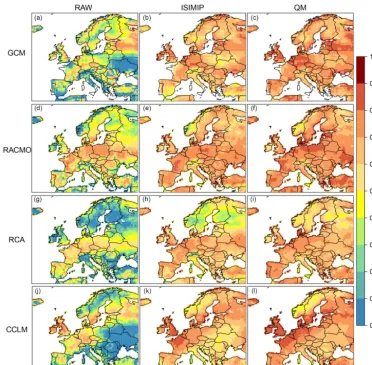
An overall conclusion about better performance is not ev-ident since the results depend on each grid box and GCM– RCM combination, and they might be affected by compen-sations for biases in the individual variables. A summary for the evaluation of the inter-variable relationships across Eu-rope is presented through the Perkins score (Fig. 6). Lower scores are apparent in the raw GCM and RCM data, espe-cially in areas with complex orography and southeastern Eu-rope. The two BC methods are able to improve the represen-tation of the inter-variable relationships on the whole conti-nent just by centring the distributions. High Perkins scores are found, especially along the Atlantic coast. QM improves on ISIMIP in large areas, although low scores are found in Scandinavia (0.7–0.8) for the RCMs. The spatial distribu-tion of the scores qualitatively agrees with biases in the tem-poral variability of maximum and dew-point temperatures (Figs. S4–S5). This is a first-order indication that the mis-representation of the temporal variability of the individual variables might be responsible for most of the deficiencies in the inter-variable relationships. Raw model data overesti-mate the temporal variability, especially in eastern Europe, leading to Perkins scores lower than 0.6. In other areas, such
as Scandinavia, the models underestimate the temporal vari-ability of the two input variables and thus present the lowest scores even after QM. The best results are obtained for GCM QM, with large scores also in northern Europe (Fig. 6c).
3.3 Future changes of heat stress
For all the models considered (GCM, RCMs and BC meth-ods) summer mean WBGT and WBGTp99 are projected to increase by the end of the 21st century under RCP8.5 (Figs. 7 and S4). For a given RCP, the major source of uncertainty in the magnitude of this change comes from the choice of GCM or RCM, with a systematically lower change signal in the RCMs. The differences in the climate change signal between the GCM and the RCMs may range between 0.5 and 1◦C, depending on the RCM and RCP, for the European averaged values. It is related to the reduced summer warming in many EURO-CORDEX RCMs with respect to their driving GCMs that was noted already in previous works, which pointed to different circulation patterns, surface energy fluxes and feed-back mechanisms as possible causes for this (Keuler et al., 2016; Sørland et al., 2018). The raw GCM projects changes in summer mean WBGT above 4.5◦C over most parts of the continent, with the highest values in the Alpine area (more than 6◦C), whereas RCMs project increases between 3 and 5◦C on most of the continent (Fig. 7; shown are RCMs at 0.11◦but similar results are found for 0.44◦). The Alps and north of Scandinavia stand out with larger positive signals. By construction, ISIMIP approximately preserves the cli-mate change signals of the input variables (Hempel et al., 2013), whereas QM can potentially modify them (e.g. Gob-iet et al., 2015; Ivanov et al., 2018; see also Sect. 2.4). Our results show that little changes become apparent for the mean WBGT after ISIMIP (up to half a degree). The effect of the QM on the WBGT signal is especially noticeable for the case of the GCM, for which QM reduces the signal by up to 1.5◦C and brings it closer to the RCM counterpart. The large pos-itive signal over the Alpine area is retained and stands out (although with smaller magnitude) for the RCM QM. Simi-lar conclusions can be drawn for the change in WBGTp99, with a slightly patchier spatial pattern (Fig. S4).
cli-Figure 6.Spatial distribution of Perkins skill scores calculated from the two-dimensional distribution of summer values of daily maximum temperature and daily mean dew-point temperature for the GCM (a–c)and the RCMs at EUR-11(d–l)for raw (first column), ISIMIP corrected (second column) and QM corrected (third column).
mate change signals and slightly lower the median for the two CCLM simulations.
The modification of the climate change signal by BC is further analysed for the grid boxes over Warsaw (Fig. 9a, b) and Madrid (Fig. 9c, d), considering the change signals in the mean variables (Fig. 9a, c) and in the 99th percentile (Fig. 9b, d). In Warsaw, QM tends to reduce the signal of the GCM and RCMs towards lower maximum temperatures (Fig. 9a). These changes in the signal are larger for the GCM than the RCMs. In this grid box, the effect of QM on mean dew-point temperature is negligible. As a consequence, the modification of the signal in mean WBGT is less than 0.5◦C for the RCMs and 1◦C for the GCM. Given that the pro-jected change for mean WBGT is 3.5–5◦C for the RCMs (∼5.5◦C for the GCM), the impact of the QM can amount to a maximum of 15 % (18 %) of the raw signal. Modifications in the climate change signal of the WBGTp99 by QM are smaller than for the mean, along with smaller changes in the signal of the 99th percentile of the input variables (Fig. 9b;
note that WBGTp99 is not necessarily linked to the 99th per-centile of maximum temperature and dew-point temperature but to some percentile in the upper tail of the distribution). In this example, however, it is evident that the preservation of trends by ISIMIP depends on the parameter under considera-tion, since e.g. the signal in the 99th percentile of dew-point temperature for CCLM-044 is reduced by 1.3◦C after the application of ISIMIP (see grey lines in Fig. 9b). Again the modifications of the climate change signal are grid box spe-cific, and negligible changes are found after QM and ISIMIP for the grid box closest to Madrid (Fig. 9c, d).
4 Summary and discussion
Figure 7.Spatial distribution of changes in summer mean WBGT under RCP8.5 for the GCM(a–c)and RCMs at EUR-11(d–l)for raw (first column), ISIMIP corrected (second column) and QM corrected (third column). The climate change signals are calculated for the period 2070–2099 with respect to 1981–2010.
added value of (1) a more complex BC method, as well as (2) bias-corrected RCM simulations versus bias-corrected GCM simulations, and (3) the role of downscaling and BC on the climate change signal of a multivariate index. For this purpose, we used GCM data from the CMIP5 HadGEM2-ES and the HadGEM-driven EURO-CORDEX simulations at approximately 12 and 50 km horizontal resolution, respec-tively. The study was performed for the case of heat stress in Europe, considering as a heat stress index the wet-bulb globe temperature (WBGT) in shaded conditions. It depends on air temperature and dew-point temperature, which were separately corrected prior to the index calculation. The per-formance of the models and methods in such a multivariate framework was analysed. The results were examined con-sidering present climate simulations (reference period 1981– 2010) and future climate projections (2070–2099).
Regarding the performance of the two bias correction methods, the evaluation results show that both methods are
Figure 8.Climate change signals for summer mean WBGT(a), daily maximum temperature (Tx,b) and daily mean dew-point temperature (Td,c) for the period 2070–2099 with respect to 1981–2010 and RCP2.6, 4.5 and 8.5. Each box represents the changes across all grid boxes in Europe for raw (blue), ISIMIP corrected (orange) and QM corrected (green) for the GCM and the RCMs (EUR-11 and EUR-44). Due to the different land–sea masks in the observations, the GCM and RCMs (EUR-44 and EUR-11), all box plots consider the grid boxes common to all data sets.
biases of the raw GCM in the inter-variable dependencies might be related to biases in large-scale processes and feed-backs. Further research is needed to understand the causes for these biases, while the application of BC for those cases in a multivariate context is then debatable (Piani et al., 2010; Ehret et al., 2012; Muerth et al., 2013). Other methods and approaches (i.e. perfect prognosis approach, high-resolution regional models) are viable alternatives to bias correction in those cases (Maraun, 2016; Maraun et al., 2017).
Regarding climate change projections of WBGT, the largest differences for a given RCP come from the use of GCM versus RCM data, with systematically lower signals
Figure 9.Scatter plots showing the effect of BC on the climate change signal for dew-point temperature (xaxis), maximum temperature (yaxis) and WBGT (coloured markers) for the grid box over Warsaw(a, b)and Madrid(c, d)for RCP8.5 and the period 2070–2099 with respect to 1981–2010. Panels(a, c)show results for the change signal of the mean variables and panels(b, d)for the 99th percentiles. Each marker depicts results for a different data set (squares for the GCM, upwards triangles for RCMs at EUR-44 and downwards triangles for RCMs at EUR-11). The black arrows point from the value in the raw data (thicker markers) to the change in the QM-corrected data, whereas the grey arrows point from the raw to the ISIMIP-corrected data (only discernible for the change signal of the 99th percentiles).
some modifications of the signal in WBGT statistics may be-come apparent after the correction. The modifications of the climate change signals due to bias correction are generally smaller than the model uncertainty (spread over the GCM and RCMs at two resolutions) by the end of the century. The magnitude of these changes should also be analysed in the context of natural variability (Räisänen, 2001), since the lat-ter can mask or enhance long-lat-term trends.
bias-corrected data qualitatively retain the change signal of the raw counterparts, although QM tends to decrease the signal of the WBGT and the input variables.
Some limitations and points for discussion remain. The use of a single GCM (even downscaled with several RCMs and bias corrected) for the production of climate projec-tions does not sample the full uncertainty range, and the use of large ensembles of simulations is strongly recom-mended. GCMs typically produce larger estimates for the change signal of temperature than RCMs due to different cir-culation patterns, surface energy fluxes and feedback mech-anisms (Keuler et al., 2016; Sørland et al., 2018). HadGEM in particular projects an increase in summer mean WBGT of 5◦C (European average, end of 21st century, RCP8.5) and HadGEM-driven RCM simulations of about 4–4.5◦C. These results are at the upper limit of the uncertainty range when compared to a large ensemble of GCM–RCM simula-tions (Casanueva et al., 2019). Therefore, relying only on this GCM could lead to misleading conclusions when combined with other factors in impact assessments. This example high-lights even further the need for ensembles of simulations.
The differences between the two RCM resolutions were negligible in our study, mainly due to the experimental de-sign (both resolutions are remapped onto the 50×50 km ob-servational grid). The higher-resolution RCMs could show some potential added value if the evaluation was carried out at their original resolution. However, there is no pan-European, high-resolution, observational grid for air tem-perature or for dew-point temtem-perature (or relative humidity) to bias correct and evaluate these simulations. While high-resolution grids for temperature are available at a national level, the lack of a gridded product for relative humidity re-mains a limitation. Furthermore, model evaluation can de-pend on the reference data set employed and observations play a fundamental role in bias correction, especially in QM for which the whole distribution is adjusted. Previous stud-ies have shown that model uncertainty dominates over obser-vational uncertainty for the case of mean temperature (Kot-larski et al., 2019a), but dew-point temperature (or relative humidity) has not been broadly investigated so far. In the present work, we do not account for observational uncer-tainty but acknowledge that the reliability and spatial rep-resentativeness of the reference data set might quantitatively modify the results. Future works also including a comparison of different observational data products might shed light on the robustness of the current results.
Code availability. All calculations and plots were produced us-ing R (https://www.r-project.org/, last access: 2 August 2019; ver-sion 3.3.2) by making use of open-source R packages. The code used for ISIMIP is part of the R package climate4R(Cofiño et al., 2018; Iturbide et al., 2019) available from a GitHub repos-itory (https://github.com/SantanderMetGroup/downscaleR; Bedia et al., 2017). In this work we used downscaleR version 3.0.3
(DOI: https://doi.org/10.1016/j.envsoft.2018.09.009; Iturbide et al., 2019). We used the R package qmCH2018 for the quan-tile mapping bias correction (https://github.com/SvenKotlarski/ qmCH2018, last access: 2 August 2019; version v1.0.1; DOI: https://doi.org/10.5281/zenodo.3275571; Kotlarski et al., 2019b). It was also used for bias correcting and downscaling within the framework of the CH2018 Swiss Climate Change Scenarios (http: //www.ch2018.ch, last access: 2 August 2019). The heat stress index was calculated with the R packageHeatStress(https://github.com/ anacv/HeatStress, last access: 2 August 2019; version v1.0.7; DOI: https://doi.org/10.5281/zenodo.3264930; Casanueva, 2019a) and all plots were produced with the R packageplotFun(https://github. com/anacv/plotFun, last access: 2 August 2019; version 1.0.5; DOI: https://doi.org/10.5281/zenodo.3265025; Casanueva, 2019b). The last two packages were developed in the framework of the Hori-zon 2020 HEAT-SHIELD project (https://www.heat-shield.eu/, last access: 2 August 2019). All the code to perform the derived anal-yses, calculations and plots is also based on R scripts, which are available upon request.
Data availability. The model simulations (EURO-CORDEX RCMs and HadGEM2-ES) used in this study are accessible via the Earth System Grid Federation (ESGF archive; https://esgf.llnl.gov, last access: 2 August 2019). The ESGF architecture consists of a global system of distributed nodes, which inter-operate with others according to a peer-to-peer paradigm; i.e. each node can act as the provider or the consumer of services. They can join or leave the federation dynamically, without affecting the operations of the other nodes. The user needs to have an OpenID and can select different search criteria. To get the RCM data used in this work the selection is as follows: Project=“CORDEX”; Domain =“EUR-11” and “EUR-44”; Experiment= “historical”, “rcp26”, “rcp45”, “rcp85”; Time Frequency = “day”; Variable = “tas”, “tasmax”, “hurs” (or “huss” and “ps”). The HadGEM2-ES data are also available through the ESGF System, selecting the search criteria: Project = “CMIP5”; Institute = “MOHC”; Model = “HadGEM2-ES”; Experiment = “historical”, “rcp26”, “rcp45”, “rcp85”; Time Frequency=“day”; Ensemble=“r1i1p1”; Variable =“tas”, “tasmax”, “huss”, “psl”.
Supplement. The supplement related to this article is available on-line at: https://doi.org/10.5194/gmd-12-3419-2019-supplement.
Author contributions. AC, SK and TK conceived the study. SH im-plemented the ISIMIP method in R, SK re-edited the QM code used in this work and AC implemented the heat stress index in R. AC per-formed the analyses, and SK and SH gave support regarding the bias correction methods and model data. AMF and CS provided ideas for new analyses and illustrations. AC wrote the first draft of the paper, and all authors reviewed the text and contributed to the final version.
Acknowledgements. The authors are grateful to the World Climate Research Programme’s Working Group on Regional Climate and the Working Group on Coupled Modelling, the former coordinat-ing body of CORDEX and the responsible panel for CMIP5. We also thank the climate modelling groups for producing and mak-ing available their model output. We also acknowledge the Earth System Grid Federation infrastructure, an international effort led by the U.S. Department of Energy’s Program for Climate Model Diagnosis and Intercomparison, the European Network for Earth System Modelling and other partners in the Global Organisation for Earth System Science Portals (GO-ESSP). We also thank Cur-din Spirig (ETH Zurich) for preprocessing the simulation data and Jan Rajczak (ETH Zurich) for providing an earlier version of the quantile mapping code. We also thank our HEAT-SHIELD col-leagues (https://www.heat-shield.eu/) and the CH2018 group (http: //www.ch2018.ch) for technical support and scientific discussions. The authors wish to thank the Swiss National Supercomputing Cen-tre (CSCS) for providing the technical infrastructure. We also thank two anonymous referees for their useful comments that helped to improve the original paper.
Financial support. This research has been supported by the Euro-pean Commission (HEAT-SHIELD (668786)).
Review statement. This paper was edited by Lauren Gregoire and reviewed by two anonymous referees.
References
Bedia, J., Gutiérrez, J. M., Herrera, S., Iturbide, M., and Manzanas, R.: downscaleR: An R package for bias correction and statisti-cal downsstatisti-caling. R package version 2.0.4, available at: https:// github.com/SantanderMetGroup/downscaleR (last access: 2 Au-gust 2019), 2017.
Bernard, T. E. and Pourmoghani, M.: Prediction of Workplace Wet Bulb Global Temperature, Applied Occupational and Environ-mental Hygiene, 14, 126–134, 1999.
Casanueva, A.: HeatStress, Zenodo, https://doi.org/10.5281/ zenodo.3264930, 2019a.
Casanueva, A.: plotFun, Zenodo, https://doi.org/10.5281/zenodo. 3265025, 2019b.
Casanueva, A., Kotlarski, S., Herrera, S., Fernández, J., Gutiérrez, J. M., Boberg, F., Colette, A., Christensen, O. B., Goergen, K., Jacob, D., Keuler, K., Nikulin, G., Teichmann, C., and Vautard, R.: Daily precipitation statistics in a EURO-CORDEX RCM en-semble: added value of raw and bias-corrected high-resolution simulations, Clim. Dynam., 47, 719–737, 2016.
Casanueva, A., Bedia, J., Herrera, S., Fernández, J., and Gutiér-rez, J. M.: Direct and component-wise bias correction of multi-variate climate indices: the percentile adjustment function diag-nostic tool, Climatic Change, 147, 411–425, 2018.
Casanueva, A., Kotlarski, S., Fischer, A. M., Flouris, A. D., Kjell-strom, T., Lemke, B., Nybo, L., Schwierz, C., and Liniger, M. A.: Escalating environmental heat exposure – a future threat for the European workforce, Reg. Env. Change, in review, 2019.
Christensen, J. H., Boberg, F., Christensen, O. B., and Lucas-Picher, P.: On the need for bias correction of regional climate change projections of temperature and precipitation. Geophys. Res. Lett., 10, L20709, https://doi.org/10.1029/2008GL035694, 2008.
Coccolo, S., Kämpf, J., Scartezzini, J.-L. and Pearlmutter, D.: Out-door human comfort and thermal stress: A comprehensive review on models and standards, Urban Climate, 18, 33–57, 2016. Cofiño, A.S., Bedia, J., Iturbide, M., Vega, M., Herrera, S.,
Fer-nández, J., Frías, M. D., Manzanas, R., and Gutiérrez J. M.: The ECOMS User Data Gateway: Towards seasonal forecast data provision and research reproducibility in the era of Climate Ser-vices, Climate SerSer-vices, 9, 33–43, 2018.
Collins, W. J., Bellouin, N., Doutriaux-Boucher, M., Gedney, N., Halloran, P., Hinton, T., Hughes, J., Jones, C. D., Joshi, M., Lid-dicoat, S., Martin, G., O’Connor, F., Rae, J., Senior, C., Sitch, S., Totterdell, I., Wiltshire, A., and Woodward, S.: Development and evaluation of an Earth-System model – HadGEM2, Geosci. Model Dev., 4, 1051–1075, https://doi.org/10.5194/gmd-4-1051-2011, 2011.
Dee, D. P., Uppala, S. M., Simmons, A. J., Berrisford, P., Poli, P., Kobayashi, S., Andrae, U., Balmaseda, M. A., Balsamo, G., Bauer, P., Bechtold, P., Beljaars, A. C. M., van de Berg, L., Bid-lot, J., Bormann, N., Delsol, C., Dragani, R., Fuentes, M., Geer, A. J., Haimberger, L., Healy, S. B., Hersbach, H., Hólm, E. V., Isaksen, L., Kaallberg, P., Köhler, M., Matricardi, M., McNally, A. P., Monge-Sanz, B. M., Morcrette, J.J., Park, B.K., Peubey, C., de Rosnay, P., Tavolato, C., Thépaut, J.-N., and Vitart, F.: The ERA-Interim reanalysis: configuration and performance of the data assimilation system, Q. J. Roy. Meteor. Soc., 137, 553–597, 2011.
de Freitas, C. R. and Grigorieva, E. A.: A comprehensive cata-logue and classification of human thermal climate indices, Int. J. Biometeorol., 59, 109–120, 2015.
Déqué, M.: Frequency of precipitation and temperature extremes over France in an anthropogenic scenario: Model results and sta-tistical correction according to observed values, Global Planet. Change, 5, 16–26, 2007.
Ehret, U., Zehe, E., Wulfmeyer, V., Warrach-Sagi, K., and Liebert, J.: HESS Opinions “Should we apply bias correction to global and regional climate model data?”, Hydrol. Earth Syst. Sci., 16, 3391–3404, https://doi.org/10.5194/hess-16-3391-2012, 2012. Fernández, J., Frías, M. D., Cabos, W. D., Cofiño, A. S.,
Domínguez, M., Fita, L., Gaertner, M. A., García-Díez, M., Gutiérrez, J. M., Jiménez-Guerrero, P., Liguori, G., Mon-távez, J. P., Romera, R., and Sánchez, E.: Consistency of cli-mate change projections from multiple global and regional model intercomparison projects. Clim. Dynam., 52, 1139, https://doi.org/10.1007/s00382-018-4181-8, 2018.
Feser, F., Rockel, B., von Storch, H., Winterfeldt, J., and Zahn, M.: Regional climate models add value to global model data: a review and selected examples, B. Am. Meteorol. Soc., 92, 1181–1192, 2011.
Fischer, E. M. and Knutti, R.: Robust projections of combined hu-midity and temperature extremes, Nat. Clim. Change, 3, 126– 130, 2013.
Ostberg, S., Popp, A., Riva, R., Stevanovic, M., Suzuki, T., Volkholz, J., Burke, E., Ciais, P., Ebi, K., Eddy, T. D., Elliott, J., Galbraith, E., Gosling, S. N., Hattermann, F., Hickler, T., Hinkel, J., Hof, C., Huber, V., Jägermeyr, J., Krysanova, V., Marcé, R., Müller Schmied, H., Mouratiadou, I., Pierson, D., Tittensor, D. P., Vautard, R., van Vliet, M., Biber, M. F., Betts, R. A., Bodirsky, B. L., Deryng, D., Frolking, S., Jones, C. D., Lotze, H. K., Lotze-Campen, H., Sahajpal, R., Thonicke, K., Tian, H., and Yamagata, Y.: Assessing the impacts of 1.5◦C global warming – simula-tion protocol of the Inter-Sectoral Impact Model Intercompar-ison Project (ISIMIP2b), Geosci. Model Dev., 10, 4321–4345, https://doi.org/10.5194/gmd-10-4321-2017, 2017.
García-Díez, M., Fernández, J., and Vautard, R.: An RCM multi-physics ensemble over Europe: multi-variable evaluation to avoid error compensation, Clim. Dynam., 2, 1–16, 2015.
Giorgi, F.: Regional climate modeling: Status and perspectives, J. Phys. IV, 12, 101–118, 2006.
Giorgi, F. and Mearns, L. O.: Approaches to the simulation of re-gional climate change: a review, RevGeo, 29, 191–216, 1991. Giorgi, F., Jones, C., and Asrar, G. R.: Addressing climate
informa-tion needs at the regional level: the CORDEX framework, WMO Bulletin, 58, 175–183, 2009.
Gobiet, A., Suklitsch, M., and Heinrich, G.: The effect of empirical-statistical correction of intensity-dependent model errors on the temperature climate change signal, Hydrol. Earth Syst. Sci., 19, 4055–4066, https://doi.org/10.5194/hess-19-4055-2015, 2015. Gutiérrez, J. M., Maraun, D., Widmann, M., Huth, R., Hertig, E.,
Benestad, R., Roessler, O., Wibig, J., Wilcke, R., Kotlarski, S., San Martín, D., Herrera, S., Bedia, J., Casanueva, A., Man-zanas, R., Iturbide, M., Vrac, M., Dubrovsky, M., Ribalaygua, J., Pórtoles, J., Räty, O., Räisänen, J., Hingray, B., Raynaud, D., Casado, M. J., Ramos, P., Zerenner, T., Turco, M., Bosshard, T., Štˇepánek, P., Bartholy, J., Pongracz, R., Keller, D. E., Fis-cher, A. M., Cardoso, R. M., Soares, P. M. M., Czernecki, B., and Pagé, C.: An intercomparison of a large ensemble of statisti-cal downsstatisti-caling methods over Europe: Results from the VALUE perfect predictor cross-validation experiment, Int. J. Climatol., 39, 3750–3785, https://doi.org/10.1002/joc.5462, 2019. Hagemann, S., Chen, C., Haerter, J. O., Heinke, J., Gerten, D., and
Piani, C.: Impact of a Statistical Bias Correction on the Projected Hydrological Changes Obtained from Three GCMs and Two Hy-drology Models, J. Hydrometeor., 3, 556–578, 2011.
Hempel, S., Frieler, K., Warszawski, L., Schewe, J., and Piontek, F.: A trend-preserving bias correction – the ISI-MIP approach, Earth Syst. Dynam., 4, 219–236, https://doi.org/10.5194/esd-4-219-2013, 2013.
Hertig, E., Maraun, D., Bartholy, J., Pongracz, R., Vrac, M., Mares, I., Gutiérrez, J. M., Wibig, J., Casanueva, A., and Soares, P. M. M.: Comparison of statistical downscaling methods with re-spect to extreme events over Europe: Validation results from the perfect predictor experiment of the COST Action VALUE, Int. J. Climatol., 39, 3846–3867, https://doi.org/10.1002/joc.5469, 2019.
Hewitson, B .C., Daron, J., Crane, R. G., Zermoglio, M. F., and Jack, C.: Interrogating empirical-statistical downscaling, Cli-matic Change, 122, 539–554, 2014.
Ioannou, L. G., Tsoutsoubi, L., Samoutis, G., Bogataj, L. K., Kenny, G. P., Nybo, L., Kjellstrom, T., and Flouris, A. D.: Time-motion analysis as a novel approach for evaluating the impact of
environ-mental heat exposure on labor loss in agriculture workers, Tem-perature, 4, 330–340, 2017.
IOM (International Organization for Migration): Extreme heat and migration, Environment and Climate Change Division, Geneva, Switzerland, 2016.
ISO: Hot environments – Estimation of the heat stress on work-ing man, based on the WBGT-index (wet bulb globe temper-ature), International Standards Organization, Geneva, Switzer-land, 1989.
ISO: Hot environments – Ergonomics of the thermal environment – Assessment of heat stress using the WBGT (wet bulb globe tem-perature) index, International Standards Organization, Geneva, Switzerland, 2017.
Iturbide, M., Bedia, J., Herrera, S., Baño-Medina, J., Fernán-dez, J., Frías, M. D., Manzanas, R., San-Martín, D., Cimadev-illa, E., Cofiño, A. S., and Gutiérrez, J. M.: The R-based climate4R open framework for reproducible climate data ac-cess and post-proac-cessing, Environ. Modell. Softw., 111, 42–54, https://doi.org/10.1016/j.envsoft.2018.09.009, 2019.
Ivanov, M. A., Luterbacher, J., and Kotlarski, S.: Climate Model Biases and Modification of the Climate Change Signal by Intensity-Dependent Bias Correction, J. Climate, 31, 6591–6610, https://doi.org/10.1175/JCLI-D-17-0765.1, 2018.
Jacob, D., Petersen, J., Eggert, B., Alias, A., Christensen, O.B., Bouwer, L. M., Braun, A., Colette, A., Déqué, M., Georgievski, G., Georgopoulou, E., Gobiet, A., Menut, L., Nikulin, G., Haensler, A., Hempelmann, N., Jones, C., Keuler, K., Kovats, S., Kröner, N., Kotlarski, S., Kriegsmann, A., Martin, E., van Mei-jgaard, E., Moseley, C., Pfeifer, S., Preuschmann, S., Raderma-cher, C., Radtke, K., Rechid, D., Rounsevell, M., Samuelsson, P., Somot, S., Soussana, J.-F., Teichmann, C., Valentini, R., Vau-tard, R., Weber, B., and Yiou, P.: EURO-CORDEX: new high-resolution climate change projections for European impact re-search, Reg. Environ. Change, 14, 563–578, 2014.
Jones, C., Giorgi, F., and Asrar, G.: The Coordinated Regional Downscaling Experiment: CORDEX, An international down-scaling link to CMIP5, CLIVAR Exchanges, 56, 34–40, 2011. Keuler, K., Radtke, K., Kotlarski, S., and Lüthi, D.: Regional
cli-mate change over Europe in COSMO-CLM: Influence of emis-sion scenario and driving global model, Meteorol. Z., 5, 121– 136, 2016.
Kjellstrom, T., Kovats, S., Lloyd, S. J., Holt, T., and Tol, R. S. J.: The direct impact of climate change on regional labour produc-tivity, Int Archives of Environmental & Occupational Health, 64, 217–227, 2009.
Kjellstrom, T., Freyberg, C., Lemke, B., Otto, M., and Briggs, D.: Estimating population heat exposure and impacts on working people in conjunction with climate change, Int. J. Biometeorol., 62, 291–306, 2018.
Koppe, C., Kovats, S., Jendritzky, G., and Menne, B.: Heat waves: risks and responses, No. 2, Health and Global Environmental Change Series, World Health Organisation, Copenhagen, Den-mark, 2004.
EURO-CORDEX RCM ensemble, Geosci. Model Dev., 7, 1297–1333, https://doi.org/10.5194/gmd-7-1297-2014, 2014.
Kotlarski, S., Szabó, P., Herrera, S., Räty, O., Keuler, K., Soares, P. M. M., Cardoso, R. M., Bosshard, T., Pagé, C., Boberg, F., Gutiérrez, J. M., Isotta, F. A., Jaczewski, A., Kreienkamp, F., Liniger, M. A., Lussana, C., and Pianko-Kluczy´nska, K.: Ob-servational uncertainty and regional climate model evaluation: a pan-European perspective, Int. J. Climatol., 39, 3730–3749, https://doi.org/10.1002/joc.5249, 2019a.
Kotlarski, S., Rajczak, J., and Feigenwinter, I.: qmCH2018, Zen-odo, https://doi.org/10.5281/zenodo.3275571, 2019b.
Lanzante, J. R., Dixon, K. W., Nath, M. J., Whitlock, C. E., and Adams-Smith, D.: Some Pitfalls in Statistical Downscaling of Future Climate, B. Am. Meteorol. Soc., 99, 791–803, 2018. Lemke, B. and Kjellstrom, T.: Calculating workplace WBGT from
meteorological data, Ind. Health, 50, 264–278, 2012.
Maraun, D.: Bias Correcting Climate Change Simulations – a Criti-cal Review, Current Climate Change Reports, 2, 211–220, 2016. Maraun, D., Wetterhall, F., Ireson, A. M., Chandler, R. E., Kendon, E. J., Widmann, M., Brienen, S., Rust, H. W., Sauter, T., Themessl, M., Venema, V. K. C., Chun, K. P., Goodess, C. M., Jones, R. G., Onof, C., Vrac, M., and Thiele-Eich, I.: Precipita-tion downscaling under climate change: Recent developments to bridge the gap between dynamical models and the end user, Rev. Geophys., 48, RG3003, https://doi.org/10.1029/2009RG000314, 2010.
Maraun, D., Shepherd, T. G., Widmann, M., Zappa, G., Walton, D., Gutiérrez, J. M., Hagemann, S., Richter, I., Soares, P. M. M., Hall, A., and Mearns, L. O.: Towards process-informed bias correction of climate change simulations, Nat. Clim. Change, 7, 764–773, 2017.
Meijgaard, E., van Ulft, L., van de Berg, W., Bosveld, B., van der Hurk, B., Lenderik, G., and Siebesma, A.: The KNMI regional atmospheric climate model RACMO version 2.1., Tech. Rep., 302, Royal Netherlands Meteorological Institute (KNMI), De Bilt, the Netherlands, 2008.
Muerth, M. J., Gauvin St-Denis, B., Ricard, S., Velázquez, J. A., Schmid, J., Minville, M., Caya, D., Chaumont, D., Lud-wig, R., and Turcotte, R.: On the need for bias correction in regional climate scenarios to assess climate change im-pacts on river runoff, Hydrol. Earth Syst. Sci., 17, 1189–1204, https://doi.org/10.5194/hess-17-1189-2013, 2013.
NIOSH: NIOSH criteria for a recommended standard: occupa-tional exposure to heat and hot environments, U.S. Department of Health and Human Services, Centers for Disease Control and Prevention, National Institute for Occupational Safety and Health, DHHS (NIOSH), Publication 2016-106, Cincinnati, OH, USA, 2016.
Nybo, L., Kjellstrom, T., Kajfez, L. K., and Flouris, A. D.: Global heating: Attention is not enough; we need acute and appropriate actions, Temperature, 4, 199–201, 2017.
Parsons, K.: Human thermal environment: The effects of hot, mod-erate and cold temperatures on human health, Third edition, CRC Press, New York, USA, 2014.
Pearson, K.: Notes on regression and inheritance in the case of two parents, P. R. Soc. London, 58, 240–242, 1895.
Perkins, S. E., Pitman, A. J., Holbrook, N. J., and McAneney, J.: Evaluation of the AR4 Climate Models’ Simulated Daily Max-imum Temperature, MinMax-imum Temperature, and Precipitation
over Australia Using Probability Density Functions, J. Climate, 20, 4356–4376, 2007.
Piani, C., Weedon, G. P., Best, M., Gomes, S. M., Viterbo, P., Hage-mann, S., and Haerter, J. O.: Statistical bias correction of global simulated daily precipitation and temperature for the application of hydrological models, J. Hydrol., 395, 199–215, 2010. Pogaˇcar, T., Casanueva, A., Kozjek, K., Ciuha, U., Mekjavic, I.B.,
Kajfez Bogataj, L., and ˇCrepinsek, Z.: The effect of hot days on occupational heat stress in the manufacturing industry: implica-tions for workers’ well-being and productivity, Int. J. Biometeo-rol., 62, 1251–1264, https://doi.org/10.1007/s00484-018-1530-6, 2018.
Prein, A. F., Gobiet, A., Truhetz, H., Keuler, K., Goergen, K., Te-ichmann, C., Fox Maule, C., van Meijgaard, E., Déqué, M., Nikulin, G., Vautard, R., Colette, A., Kjellström, E., and Jacob, D.: Precipitation in the EURO-CORDEX 0.11◦and 0.44◦ simu-lations: high resolution, high benefits?, Clim. Dynam., 46, 383– 412, https://doi.org/10.1007/s00382-015-2589-y, 2016. Räisänen, J.: CO2-Induced Climate Change in CMIP2 Experiments:
Quantification of Agreement and Role of Internal Variability, J. Climate, 14, 2088–2104, 2001.
Rajczak, J., Kotlarski, S., Salzmann, N., and Schär, C.: Robust cli-mate scenarios for sites with sparse observations: a two-step bias correction approach, Int. J. Climatol., 36, 1226–1243, 2016. Rockel, B., Will, A., and Hense, A.: The Regional Climate Model
COSMO-CLM (CCLM), Meteorol. Z., 17, 347–348, 2008. Samuelsson, P., Jones, C. G., Willén, U., Ullerstig, A.,
Gol-lvik, S., Hansson, U., Jansson, C., Kjellström, E., Nikulin, G., and Wyser, K.: The Rossby Centre Regional Climate model RCA3: model description and performance, Tellus A, 63, 4–23, https://doi.org/10.1111/j.1600-0870.2010.00478.x, 2011. Sørland, S. L., Schär, C., Lüthi, D., and Kjellström, E.: Bias
pat-terns and climate change signals in GCM-RCM model chains, Environ. Res. Lett., 13, 074017, https://doi.org/10.1088/1748-9326/aacc77, 2018.
Taylor, K. E., Stouffer, R. J., and Meehl, G. A.: An Overview of CMIP5 and the Experiment Design, B. Am. Meteorol. Soc., 93, 485–498, 2011.
Themeßl, M. J., Gobiet, A., and Heinrich, G.: Empirical-statistical downscaling and error correction of regional climate models and its impact on the climate change signal, Climatic Change, 112, 449–468, 2012.
UNDP/ILO: Climate change and Labour: impacts of heat in the workplace, CVF Secretariat, United Nations Development Pro-gram, Geneva, Switzerland, 2016.
VividEconomics: Impacts of higher temperatures on labour produc-tivity and value for money adaptation: lessons from five DFID priority country case studies, London, UK, 2017.
Warrach-Sagi, K., Schwitalla, T., Wulfmeyer, V., and Bauer, H.-S.: Evaluation of a climate simulation in Europe based on the WRF– NOAH model system: precipitation in Germany, Clim. Dynam., 41, 755–774, 2013.
Warszawski, L., Frieler, K., Huber, V., Piontek, F., Serdeczny, O., and Schewe, J.: The Inter-Sectoral Impact Model Intercompar-ison Project (ISI–MIP): Project framework, P. Natl. Acad. Sci. USA, 111, 3228–3232, 2014.
WATCH Forcing Data methodology applied to ERA-Interim re-analysis data, Water Resour. Res., 50, 7505–7514, 2014. Wilby, R. L. and Dessai, S.: Robust adaptation to climate change,
Weather, 65, 180–185, 2010.