A Statistical Analysis of Gauss-Seidel Algorithm

(1)

Anale. Seria Informatică. Vol. VIII fasc. 2 – 2010 Annals. Computer Science Series. 8th_{Tome 2}nd_{Fasc. – 2010}

A

S

t

a

t

i

s

t

i

c

a

l

A

n

a

l

y

s

i

s

o

f

G

a

u

s

-

S

e

i

d

e

l

A

l

g

o

r

i

t

h

m

D

DiivvyyaaNNuuppuurrMMooddii

Department of Computer Science and Engineering, BIT Mesra, Ranchi, 835215, India

S

SoouubbhhiikkCChhaakkrraabboorrttyy

Department of Applied Mathematics, BIT Mesra, Ranchi, 835215, India

ABSTRACT: The paper statistically analyzes Gauss Seidel method of solving a system of linear equations AX=B, involving n variables and n independent linear equations, when A and B are filled with random numbers from discrete uniform [1, 2, 3,…k] variates. It is observed that the number of iterations (r) can be predicted by a third degree polynomial in n, independent of k.

KEYWORDS: Gauss-Seidel method; Chebyshev’s inequality; Chi-square statistic; regression; discrete uniform distribution.

Introduction

Gauss-Seidel Method: It is an iterative technique used to solve a linear system of equations. It is defined on matrices with non-zero diagonals, convergence is only guaranteed if the matrix is either diagonally dominant or symmetric and positive definite. This method is an improvement on the Jacobi method.

For solving a set of linear equations, expressed in matrix term as

AX=B, the Gauss-Seidel iteration is:

X(k+1)=(D+L)-1(B-UX(k)),

(2)

When implementing Gauss-Seidel, an explicit entry-by-entry approach is used:

Xi(k+1)=

where, i = 1,2,…,n.

Note: computation of Xi(k+1) uses only those elements that have already been computed and only those elements of X(k) that have yet to be advanced to iteration k+1.This means that no additional storage is required and the computation can be done in place(X(k+1) replaces X(k)).

For more literature on Gauss-Seidel method, see [wik**]. The following points are important:

1. The convergence of the Jacobi method does not imply the convergence of the Gauss-Seidel method. The converse is also not true. But, if A is diagonally dominant, then the Gauss-Seidel method converges more rapidly than the Jacobi method.

2. The condition that A must be strictly dominant is sufficient but not necessary for the convergence i.e. there exist systems of equations which are not strictly diagonally dominant but converge.

3. The number of arithmetical operations is r.n2, where r is the number of iterations required for some specified convergence criteria and n is the number of equations. See [RS04] and references cited therein.

1.1 Empirical analysis of Gauss-Seidel Method

We raise and answer three questions:

1. If A and B are filled with random numbers from discrete uniform distribution in the range [1, 2, 3, …k], does the no. of iterations(r) depend on k?

2. Can we determine the probability distribution of r experimentally, in case of convergence, for a given n? (this settles the cases for fixed n about which we may be having some prior information in a specific case study)

3. What empirical model should we use to predict r in terms of n? (here n is a variable that serves as a predictor in a regression model; thus this study is very valuable as it covers cases where we do not have

( 1) ( )

1

(

k k

)

j j

i ij ij

ii _{j i} _{j i}

B

a

_X

a

_X

a

+

−

< >

−

(3)

any prior information about n which depends on the problem in hand and at different instances, we are getting problems with different n) In our first study, the size of matrix i.e. n is fixed at 4. Note that we could get convergence by first filling the coefficient matrix A randomly and then letting the diagonal elements have the maximum of the randomly filled elements. The vector B on the right hand side of the matrix equation was simply filled randomly without any further change. See table 1 and fig 1.

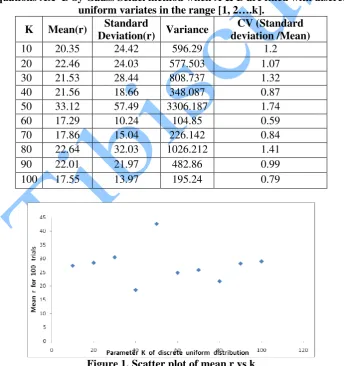
1.2 Experimental results

Table 1. Experimental results on no. of iterations r for solving the system of equations AX=B by Gauss Seidel method when A & B are filled with discrete

uniform variates in the range [1, 2….k].

K Mean(r) Standard

Deviation(r) Variance

CV (Standard deviation /Mean)

10 20.35 24.42 596.29 1.2

20 22.46 24.03 577.503 1.07

30 21.53 28.44 808.737 1.32

40 21.56 18.66 348.087 0.87

50 33.12 57.49 3306.187 1.74

60 17.29 10.24 104.85 0.59

70 17.86 15.04 226.142 0.84

80 22.64 32.03 1026.212 1.41

90 22.01 21.97 482.86 0.99

100 17.55 13.97 195.24 0.79

(4)

Interpretation

• It is clear from table1and the corresponding fig1 that there is no

pattern which can suggest that r depends on k.

• So, it appears that it is not a case of parameterized complexity. Had

it been, we might use the concept of empirical estimate to estimate the bound on r as a function of k over a finite feasible range.

• But such a possibility is not ruled out for non-uniform inputs. We

will now answer the second question.

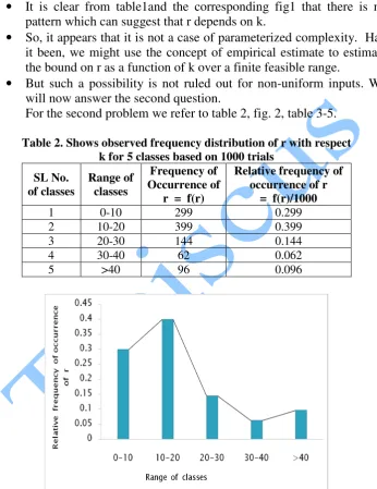
For the second problem we refer to table 2, fig. 2, table 3-5.

Table 2. Shows observed frequency distribution of r with respect k for 5 classes based on 1000 trials

SL No. of classes

Range of classes

Frequency of Occurrence of

r = f(r)

Relative frequency of occurrence of r

= f(r)/1000

1 0-10 299 0.299

2 10-20 399 0.399

3 20-30 144 0.144

4 30-40 62 0.062

5 >40 96 0.096

(5)

Interpretation

• It is clear from table2 that there is nearly 30% chance that r lies in

the range 0-10 and about 40% chance that it lies in the range 10-20.

• It is also clear from fig2 that the distribution of r is positively

skewed (right tail longer as mean exceeds mode).

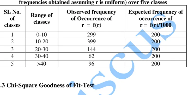
Table 3. Comparison of observed and expected frequencies of r (expected frequencies obtained assuming r is uniform) over five classes

SL No. of classes

Observed frequency of Occurrence of

r = f(r)

Expected frequency of occurrence of

r = f(r)/1000

1 0-10 299 200

2 10-20 399 200

3 20-30 144 200

4 30-40 62 200

5 >40 96 200

1.3 Chi-Square Goodness of Fit-Test

The Chi-square test is used to test if a sample of data came from a population with a specific distribution. The basic idea behind the chi-square goodness of fit test is to divide the range of the data into a number of intervals. Then the number of points that fall into each interval is compared to expected number of points for that interval if the data in fact come from the hypothesized distribution.

The primary advantage of the chi square goodness of fit test is that it is quite general. It can be applied for any distribution, either discrete or continuous, for which the cumulative distribution function can be computed. Data plot supports the chi-square goodness of fit test for all distributions for which it supports a CDF function.

Definition:

The chi-square test is defined for the hypothesis:

H0: Distribution of r is uniform over the five classes.

Hi: Distribution of r is non-uniform over the five classes.

(6)

Our test statistic follows Chi-square distribution with 4 degree of freedom where one degree of freedom is lost due to the restriction ∑Oi=∑Ei.

Table value of Chi-square at 4df and 5% level of significance= 9.488

Calculated 2 _{= 411.99}

Since calculated Chi-Squareexceeds table value of Chi- square, therefore Ho is rejected at 5% level of significance. In other words r is not uniformly distributed over the five classes. Since r does not depend on k we have pooled all the 1000 values of r taking all classes together and obtained sample estimates of mean and standard deviation of r as under:

Mean of r =21.64

Standard Deviation of r = 27.91

1.4 Chebyshev’s Inequality

It states that in any data sample or probability distribution nearly all values are close to the mean value and provides a quantitative description of “nearly all” and “close to”.

According to this:

P (E(r) - kσr ≤ r ≤ E(r)+kσr ) ≥ 1- 1/k2

The strength of this inequality is that it does not depend on the distribution of r.

If we take k=3 and substitute in the above equation we will get: P (E(r) - 3σr ≤ r ≤ E(r) +3σr) ≥ 8/9

P (21.64– 3×27.91≤ r ≤21.64 + 3×27.91) ≥ 90% (approx) Since, r represents no. of iterations, it cannot be negative Thus, P (0<r<105) ≥ 90% so long as there is convergence.

Test Statistic:

For the chi-square goodness-of-fit computation, the data are divided into k parts and the test statistic is defined as

(7)

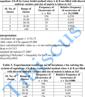
Table 4. Experimental results on no. of iterations r for solving the system of equations AX=B by Gauss Seidel method when A & B are filled with discrete

uniform variates and size of matrix is taken as 3x3

SL No. of classes

r = f(r)

Relative frequency of occurrence of

r = f(r)/1000

1 0-10 578 0.578

2 10-20 310 0.310

3 20-30 55 0.055

4 30-40 21 0.022

5 >40 36 0.036

Interpretation

Calculated chi square = 1174.73 Table value of Chi-square=9.488

Since calculated>table value so, r is not uniformly distributed. Mean r=14.313

Standard deviation=27.2007

Applying Chebyshev’s inequality for k=3, we get P(0<r<95)≥90%

Table 5. Experimental results on no. of iterations r for solving the system of equations AX=B by Gauss Seidel method when A & B are filled

with discrete uniform variates and size of matrix is taken as 5x5

SL No. of classes

r = f(r)

Relative frequency of occurrence of

r = f(r)/1000

1 0-10 106 0.106

2 10-20 393 0.393

3 20-30 185 0.185

4 30-40 90 0.09

(8)

Interpretation

Calculated chi square = 295.43 Table value of Chi-square=9.488

Since calculated>table value so, r is not uniformly distributed. Mean r=43.905

Standard deviation=90.574

Applying Chebyshev’s inequality as before, we get P(0<r<315)≥90%

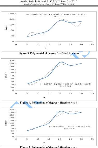
We infer that in cases where n is fixed, it is possible to experimentally determine the probability distribution of r and that even a slight change in n drastically changes the interval of r for the same probability coefficient. We are therefore motivated to fit a regression model with r as response and n as predictor. Our results suggest that a third degree polynomial is the simplest empirical model that is just adequate. Since a mathematical bound can also be estimated just like a statistical bound, except that the estimate has to be count based and operation specific, we can say that average r is empirically O(n3). The experimental results are given in table 6. For more on empirical O, see references [CS07a], [CS07b] and [C+07].

Table 6. Behavior of r versus n

n Mean(r) Standard Deviation(r) 5 42.63 65.032 10 69.45 137.99 15 100.82 346.92 20 187.44 606.35 25 168.29 471.18 30 181.73 531.091

(9)

Figure 3. Polynomial of degree five fitted to r vs n

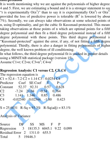
Figure 4. Polynomial of degree 4 fitted to r vs n

(10)

Interpretation

It is worth mentioning why we are against the polynomials of higher degree, 4 and 5. First, we are estimating a bound and it is a stronger statement to say “r is experimentally O(n3)” than to say it is experimentally O(n4) or O(n5) provided the loss of predictive power is tolerable (R2 is lowered by about 7%). Secondly, we can always take observations at some selected points of n, using D-optimality, and get the cubic fit Kussmaul-protected. This means taking observations at those points of n which are optimal points for a fifth degree polynomial and then fit a third degree polynomial instead of a fifth degree polynomial with these points. This third degree polynomial is “Kussmaul-protected” against the error, if any, of not fitting a fifth degree polynomial. Thirdly, there is also a danger in fitting polynomials of higher degree, the well known problem of ill conditioning.

In what follows, the third degree polynomial fit is studied in greater details using a MINITAB statistical package (version 15).

Assume C1=r; C2=n; C3=n2; C4=n3

Regression Analysis: C1 versus C2, C3, C4

The regression equation is

C1 = 52.4 - 7.2 C2 + 1.14 C3 - 0.0254 C4 Predictor Coef SE Coef T P Constant 52.37 92.31 0.57 0.628 C2 -7.24 21.04 -0.34 0.764 C3 1.141 1.346 0.85 0.486 C4 -0.02540 0.02544 -1.00 0.423

S = 25.6031 R-Sq = 93.3% R-Sq(adj) = 83.1%

Analysis of Variance

Source DF SS MS F P

Regression 3 18135.3 6045.1 9.22 0.099 Residual Error 2 1311.0 655.5

Total 5 19446.3

Durbin-Watson statistic = 3.50589.

(11)

30 25 20 15 10 5 200 175 150 125 100 75 50 C2 C 1 S 25.6031 R-Sq 93.3% R-Sq(adj) 83.1%

Fitted Line Plot

C1 = 52.37 - 7.24 C2 + 1.141 C2**2 - 0.02540 C2**3

Figure 6. Third degree polynomial fit of C1=r versus C2=n

40 20 0 -20 -40 99 90 50 10 1 Residual P e r c e n t 200 150 100 50 20 10 0 -10 -20 Fitted Value R e s id u a l 30 20 10 0 -10 -20 2.0 1.5 1.0 0.5 0.0 Residual F r e q u e n c y 6 5 4 3 2 1 20 10 0 -10 -20 Observation Order R e s id u a l

Normal Probability Plot Versus Fits

Histogram Versus Order

Residual Plots for C1

(12)

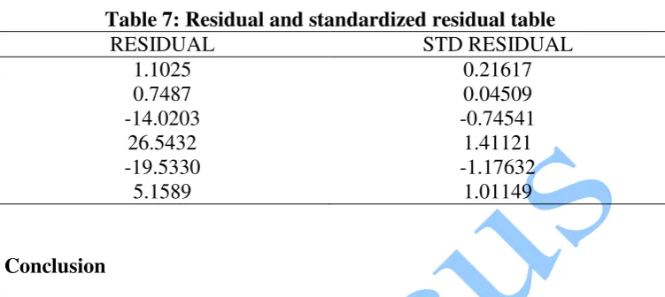
Table 7 gives the residuals and the standardized residuals.

Table 7: Residual and standardized residual table

RESIDUAL STD RESIDUAL

1.1025 0.7487 -14.0203

26.5432 -19.5330

5.1589

0.21617 0.04509 -0.74541

1.41121 -1.17632

1.01149

Conclusion

We conclude that there is nothing to confirm that r depends on k. However, we can certainly find the probability distribution of r for a fixed n experimentally. Also, for varying n, r can be predicted by a third degree polynomial in n. Our future work would cover the following points. We propose to consider the case of non-uniform input and see whether we can discover any problem of parameterized complexity in which case we may be interested in estimating a bound on r in terms of parameters of the input distribution by running computer experiments over finite feasible range. We propose to work directly on time and estimate the average complexity using statistical bound. We also look forward to support our experimental findings with corresponding theoretical analysis.

References

[CS07a] S. Chakraborty, S. K. Sourabh - On Why an Algorithmic Time Complexity Measure can be System Invariant rather than System Independent, Applied Math. and Compu, Vol. 190(1), 2007, p. 195-204

(13)

[C+07] S. Chakraborty, C. Wahi, S. K. Sourabh, L. R. Saraswati, A. Mukherjee - On the Philosophy of Statistical Bounds: A Case Study on Determinant Algorithm, Jour. of Modern Math. and Stat., Vol. 1(1-4), 2007, 15-23

[FLS06] K. T. Fang, R. Li, A. Sudjianto - Design and Modeling of Computer Experiments, Chapman and Hall, 2006

[RS04] S. B. Rao, C. K. Santha - Numerical Methods with Programs in BASIC, FORTRAN, Pascal and C++, Revised ed., Univ. Press (India) Pvt. Ltd, 2004