Steel Buildings Damage Classification by damage spectrum and Decision Tree Algorithm

(1)

journal homepage: http://civiljournal.semnan.ac.ir/

Steel Buildings Damage Classification by Damage

Spectrum and Decision Tree Algorithm

S. A. H. Hashemi1, Gh. Ghodrati Amiri2* and F. Hamedi3

1. Department of Civil Engineering, Science and Research Branch, Islamic Azad University, Tehran, Iran. 2. Professor, School of Civil Engineering Iran University of Science & Technology.

3. Assistant Professor, Faculty of Engineering, Imam Khomeini International University, Qazvin, Iran.

Corresponding author: [email protected]

ARTICLE INFO ABSTRACT

Article history:

Received: 26 January 2015 Accepted: 9 June 2015

Results of damage prediction in buildings can be used as a useful tool for managing and decreasing seismic risk of earthquakes. In this study, damage spectrum and C4.5 decision tree algorithm were utilized for damage prediction in steel buildings during earthquakes. In order to prepare the damage spectrum, steel buildings were modeled as a single-degree-of-freedom (SDOF) system and time-history nonlinear analysis was carried out to develop a set of SDOF structures. Then, damage index was used to prepare the damage spectrum. Data parameters required for training and evaluating the C4.5 decision tree algorithm were obtained from the results of damage spectra for steel structures and using Krawinkler damage index Also, two decision trees were trained based on quantitative indices. The first decision tree determined whether damage occurred in buildings or not and the second predicted severity of damage as repairable, beyond repair, or collapse. decision tree classification algorithm was used to predict damage to steel structures.

Keywords:

Damage prediction, Damage index, Steel buildings,

Decision tree algorithm.

1. Introduction

Correct prediction of damage level is very useful in estimating seismic vulnerability of buildings. Results obtained from damage prediction in structures can be effectively used to manage earthquake-caused risks. Since equivalent single-degree-of-freedom (SDOF) systems have a considerable role in

(2)

necessary to introduce some indices for evaluating damage rate on structural elements. Previous studies have proposed some damage indices as the parameters which determine damage level for structures. Results of studies have presented these indices as appropriate parameters for evaluating the damage imposed on structures, which has found widespread applications. Structural damage estimation is performed by considering usability of buildings, assumed damage function, and characteristics of the studied structure using different concepts and methods with physical interpretation capability[2]. Methods of defining a damage index at structural level are presented in 4 general forms including strength need (within elastic and non-elastic regions) [3], ductility need, energy loss[4] , and stiffness reduction [5]. A useful method for damage prediction is to calculate damage index (DI); when it is 0, the structure will remain in the elastic mode and, if it is more than 1, the structure will completely collapse. [6] The main problem with most of these methods is use of numerical values, instead of non-numerical and qualitative values, for introducing damage level.

Thus far, many functions have been proposed for determining structural damage mode after an earthquake[7]. Some of these functions are defined based on combined effects of maximum plastic displacement and plastic energy, among which is the model proposed by Baik et al. (1988) for damage evaluation in steel frames. This model utilizes Coffin - Manson relation, and Miner's rule in linear damage accumulation to achieve the behavior of structural elements [8].

In addition, Bozorgnia and Bertero proposed two modified damage indices for an SDOF non-elastic system. [6].

Dipasquale and Cakmak (1990) defined a maximum norm for a 1-D mode. This index is among the indices which are based on structural modal parameters. [9].

Damage index introduced by Ghobara et al. (1999) is adjusted by stiffness parameter and calculated by performing two pushover analyses. The first and second pushover analyses are performed before and after earthquake application to structures, respectively. This index is calculated based on structural stiffness before and after earthquake. [8]

McCabe and Hall (1989) presented a damage index based on a hysteresis behavior and equivalent ideal behavior. [10]

There are various types of damage functions; however, Krawinkler and Zohrei's damage index is often used for steel structures.

Basic relation of Krawinkler index is shown in Eq. (1):

D = ∑ 1 _N

fi

⁄ = C ∑ (Δδn _pi)c i=1

n

i=1 (1)

Where

Nfi= xA−1(Δδpi)−a = C−1(Δδpi)−c (2)

(3)

and plastic deformations is shown in Eq. (3) based on Manson-Coffin studies. [11]

𝑁𝑓= 𝐶−1(∆𝛿𝑝𝑖)−𝐶 (3)

When preparing damage spectra, a function must be defined for damage index; in this study, Krawinkler damage function was used.

2. Damage spectrum and Damage

attenuation

relations

of

steel

buildings

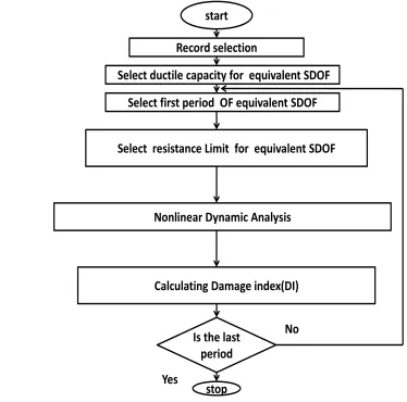
In order to determine damage level of a structure, instead of calculating velocity or acceleration spectra, damage spectrum can be directly calculated. Damage spectrum is a nonlinear spectrum which is drawn by adjusting nonlinear parameters relating to SDOF structures, performing dynamic analysis under specific records, and measuring damage for each structure. A

well-defined damage index has a normal value; if a structure remains elastic, its value will be 0 and, if there is a structural collapse potential, it will be 1. Calculation steps of damage spectrum are as follows:

1- Selecting a series of SDOF systems with period T and specific strength, force-displacement relation, and deformation;

2- Selecting a record with specific soil situation;

3- Performing nonlinear dynamic analysis;

4- Calculating damage level using dynamic analysis response and appropriate damage index; and

5- Drawing damage spectrum for different records. [6]

(4)

Select first period OF equivalent SDOF

Calculating Damage index(DI) Select ductile capacity for equivalent SDOF

Nonlinear Dynamic Analysis

Is the last

period

stop start Record selection

No

Yes

Select resistance Limit for equivalent SDOF

Figure 1. Computation of damage spectrum Damage spectrum can be calculated by the

above-introduced method. By selecting an appropriate function for damage reduction model, its coefficients are obtained using nonlinear multivariate regression method along with data from damage spectrum; then, they can be directly used to evaluate damage in different zones of a region and plan to reinforce them. Damage attenuation relations are in the form of acceleration and velocity attenuation relations:

𝐷𝐼 = 𝑓(𝑀)𝑓(𝑅) (4)

in which damage is defined as a function of magnitude and distance.

(5)

3. Record characteristics for the

applied earthquakes

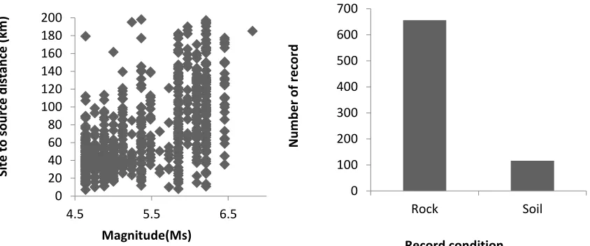
In this study, records from Building and Housing Research Center [12] were used. Since the number of records registered in Iran was more than 2000 and the number of reliable records in terms of geological

characteristics was limited, 744 records were selected, 108 records of which were related to soil conditions and 634 belonged to rock conditions. Furthermore, in this study, seismic records with the magnitude of 4.5 to 7 were used and the distance to the earthquake location was between 10 and 200 km. Characteristics of the records used in this study are shown in Fig. 2.

Figure 2. Distribution of the magnitude and distance of earthquake records

4. Calculating damage index

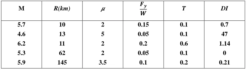
In this study, Eq. 1 was used to calculate damage index. Structural parameters used to prepare damage spectra are presented in Table 1. Also, damage index was calculated

by performing 79110 and 14580 nonlinear dynamic analyses for rock and soft soil conditions, respectively.

Table 1. Structural characteristics of steel buildings for making damage spectra

Moreover, Table 2 shows damage levels of some samples of structures with determined structural parameters under the records with specific surface magnitude (M) and focal distance (R). In this table, 𝜇, Fy/w, T, and DI

are ductility, ratio of base shear to weight, indicator of structural strength, structure's period, and damage obtained for the equivalent SDOF structure from Krawinkler damage function, respectively. In this article,

0 100 200 300 400 500 600 700

Rock Soil

N

u

m

b

e

r

o

f r

e

co

rd

Record condition

0 20 40 60 80 100 120 140 160 180 200

4.5 5.5 6.5

Si

te

t

o

so

u

rc

e

d

istan

ce

(

km

)

Magnitude(Ms)

(µ)

𝑭𝒚

𝑾

Period ( 𝑻 )

2 , 3.5, 5 0.05 , 0.1, 0.15, 0.2 , 0.3

(6)

using the above-mentioned data and decision tree method, damage was classified based on

structural characteristics and earthquake magnitude and distance to the site. [13]

Table 2. Calculating damage index for the buildings with specific structural characteristics under the effect of different earthquake records

5. Classifying values of damage

index

According to the initial definition of damage index, if DI value exceeds 1, the structure is assumed to be completely collapsed. In other words, DI of more than 1 shows collapse of the building. Thus, DI values of more than 1 in the regression analysis of reduction relations, which defines the relationship between characteristics of land movement, structural characteristics, and damage, are considered outliers. To overcome this problem, non-numerical and qualitative interpretations based on decision tree method, instead of numerical quantities, were applied to study damage prediction. [2]

Qualitative values for the building are given in Table 3. If DI is less than and equal to 0.4, the damage to the structure will be repairable and the building is slightly damaged. If DI lies between 0.4 and 1, the damage will be beyond repair and high damage is made to the building in terms of repair costs; even some parts of the building are destroyed during the earthquake. DI of larger than 1 indicates that the building is completely collapsed and cannot be occupied. These three classes of building conditions are very important for security management of the society and damage prediction algorithm in this study. Table 3 demonstrates some samples of damage classification based on performance level.

Table 3. Some samples of damage classification of the structures with specific structural parameters under different earthquake records

Damage class 𝑻

𝑭_𝒚 𝑾

𝜇

R(km) M

instance

Beyound repair

collapse

No damage

Repairable 0.1

0.1

0.6

0.1

0.2 0.15

0.05

0.2

0.05

0.1 2

5

2

3.5 10

13

11

62

145 5.7

4.6

6.2

5.3

5.9

𝐼₁ 𝐼2

𝐼₃ 𝐼₄ 𝐼5

DI 𝑻

𝑭_𝒚 𝑾

𝜇

R(km)

M

0.7

47

1.14

0

0.21 0.1

0.1

0.6

0.1

0.2 0.15

0.05

0.2

0.05

0.1 2

5

2

3.5 10

13

11

62

145 5.7

4.6

6.2

5.3

(7)

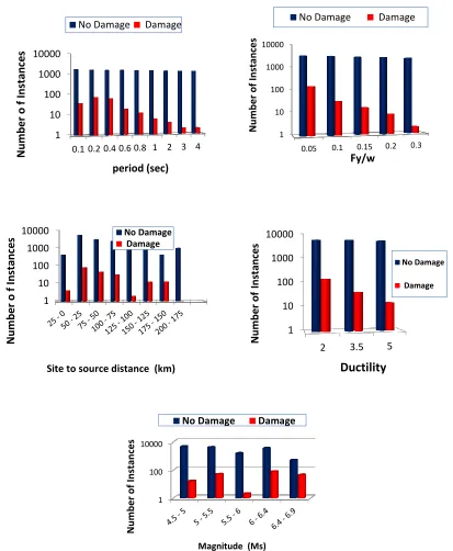
In this study, a set of data, including earthquake parameters and structural characteristics, was considered as input data. To identify structural vulnerability, decision tree algorithm was applied as the predictor

algorithm. Characteristics and distribution of this set of input data used for training the decision tree algorithm are shown in Figs. 3-6.

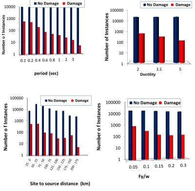
Figure 3. Distribution of 5 input characteristics of decision trees based on two outputs of damage and No damage for rock conditions

1 10 100 1000 10000

0.05 0.1 0.15 0.2 0.3

N

u

m

b

e

r

o

f In

stan

ce

s

Fy/w

No Damage Damage

1 10 100 1000 10000

0.1 0.2 0.4 0.6 0.8 1 2 3 4

N

u

mbe

r

o

f

In

sta

n

ce

s

period (sec)

No Damage Damage

1 10 100 1000 10000

N

u

mbe

r

o

f

In

sta

n

ce

s

Site to source distance (km)

No Damage Damage

1 10 100 1000 10000

2 3.5 5

Numbe

r

o

f

Ins

ta

nce

s

Ductility

No Damage

Damage

1 100 10000

N

u

m

b

e

r

o

f In

stan

ce

s

Magnitude (Ms)

(8)

Figure 4. Distribution of 5 input characteristics of decision trees based on two outputs of damage and No damage for soil conditions

1 10 100 1000 10000

0.1 0.2 0.4 0.6 0.8 1 2 3

N

um

ber

o

f

Inst

a

nce

s

period(sec)

1 10 100 1000 10000 100000

2 3.5 5

Nu

mb

er

o

f Inst

ances

Ductility

1 10 100 1000 10000 100000

N

u

mbe

r

o

f

In

sta

n

ce

s

1 10 100 1000 10000 100000

0.05 0.1 0.15 0.2 0.3

N

u

mbe

r

o

f

In

sta

n

ce

s

Fy/w

1 10 100 1000 10000 100000

N

u

m

b

e

r

o

f In

stan

ce

s

Magnitude (Ms)

(9)

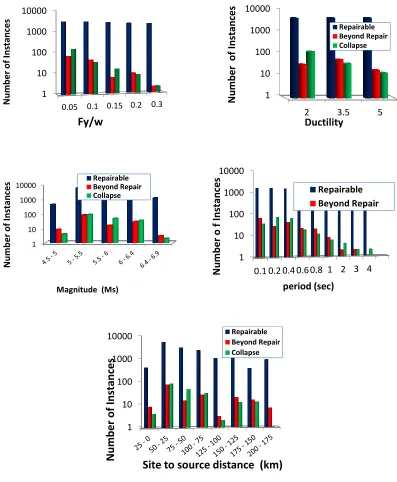
Figure 5. Distribution of 5 input characteristics of decision trees based on three outputs of repairable damage, beyond repair damage, and total collapse for soil conditions

1 10 100 1000 10000

0.05 0.1 0.15 0.2 0.3

N

u

m

b

e

r

o

f In

stan

ce

s

Fy/w

1 10 100 1000 10000

2 3.5 5

N

u

mbe

r

o

f I

n

sta

n

ce

s

Ductility Repairable Beyond Repair Collapse

1 10 100 1000 10000

Nu

m

b

er

of In

stanc

es

Magnitude (Ms) Repairable Beyond Repair Collapse

1 10 100 1000 10000

0.1 0.2 0.4 0.6 0.8 1 2 3 4

N

umber

o

f

Ins

tanc

es

period (sec)

Repairable Beyond Repair

1 10 100 1000 10000

Nu

m

b

e

r

of

In

st

an

ces

(10)

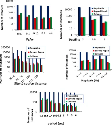
Figure 6. Distribution of 5 input characteristics of decision trees based on three outputs of repairable damage, beyond repair damage, and total collapse for rock conditions

6. Decision tree algorithm

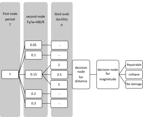
Decision trees are generated by the algorithms which divide a dataset into the parts similar to tree branches. A decision tree has a node (root) in the top part of the tree. An example of a decision tree is presented in Fig. 7. In this figure, it is obvious that a decision tree can have both discrete

(non-numerical) and continuous (numerical) properties. The relationship between the desired analyses, which act as the objective background of data, and those data acting as input data is used to develop a decision rule as a branch or different parts in the root subset. When the relation is configured, one or several decision rules can be extracted from the relationship between input data and objectives. [14]. 1 10 100 1000 10000 100000

0.05 0.1 0.15 0.2 0.3

N u m b e r o f In stan ce s Fy/w 1 10 100 1000 10000

2 3.5 5

N u m b er o f I n st an ces Ductility Repairable Beyond Repair Collapse 1 10 100 1000 10000 100000 Nu m b e r of In st an ces

Site to source distance …

Repairable Beyond Repair Collapse 1 10 100 1000 10000 100000 N u m b e r o f In stan ce s

Magnitude (Ms) Repairable Beyond Repair Collapse 1 100 10000

0.1 0.2 0.4 0.6 0.8 1 2 3 4

N u mbe r o f In sta n ce s

period (sec)

(11)

Figure 7. An example of a decision tree

There are numerous algorithms for generating decision trees. In this article, C4.5 training algorithm was used as a recognized statistical classification algorithm. C4.5 algorithm generates decision trees from a dataset using data entropy principle. Generally, the theory of data entropy principle is the measurement of irregular relationship between different and random values. Since this article did not intend to enter the details of this mathematical concept, interested readers are referred to

[15] for more information. In general terms, the purpose of this article was data mining and separating datasets for developing damage prediction decision trees using WEKA software [16]. In order to reduce prediction error in the desired decision trees, damage prediction method was performed during two phases using the relations between damage index values and damage level in steel buildings. In the first phase, two decision trees classified the structure's conditions into two non-damaged and third node

ductility µ second node

Fy/w=ABI/R First node

period T

T

0.05 ...

0.1 ...

0.15

2

3.5

decision node

for distance

decision node for magnetude

Repairable

collapse

No damage

5

0.2 ...

(12)

damaged groups. Finally, during the second phase, damage was classified into three repairable, beyond repairable, and complete collapse classes. Each pair of decision trees was developed for both soil and rock conditions. [2].Decision trees for soil and rock conditions were generated using WEKA software [16].

7. Performance of decision tree

algorithms

Purpose of generating a decision tree is to provide a decision-making tool for predicting future results in a precise way. Performance of a decision tree is evaluated based on the validity of classified records. As shown in Table 5, performance of a decision tree is generally presented as a 2×2 matrix called confusion matrix. The rows of this matrix are related to real results, while the columns show the results obtained from the classification of each class. In the field of artificial intelligence, confusion matrix refers to the matrix which demonstrates the performance of the related algorithms. Although this presentation is typically used for supervised learning algorithms, it is used in unsupervised learning algorithms as well. When this matrix is used in unsupervised learning algorithms, it is usually called

(13)

Table 4. Confusion matrix for damage and no-damage classes for soil

Table 5. Confusion matrix for damage and no-damage classes for rock

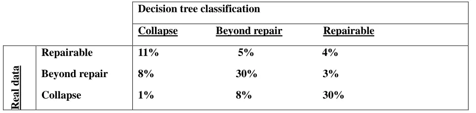
Table 6. Confusion matrix for repairable, beyond repair, and collapse classes for soil

Table 7. Confusion matrix for repairable, beyond repair, and collapse classes for rock

Decision tree classification

Damage No Damage

0.71% 4%

5% 20% No Damage

Damage

R

eal

da

ta

Damage No Damage

73% 3%

3% 22% No amage

Damage

R

eal

da

ta

Collapse Beyond repair Repairable

11% 5% 4%

8% 30% 3%

1% 8% 30% Repairable

Beyond repair

Collapse

R

eal

da

ta

Collapse Beyond repair Repairable

25% 6% 4%

7% 12% 5%

2% 4% 45% Repairable

Beyond repair

Collapse

R

eal

da

(14)

8. Validity of decision trees

Damage results obtained from time-history nonlinear analyses and decision trees for three buildings with different structural characteristics were compared with each other. Time-history nonlinear analyses were carried out considering different Fy/W ratios (0.3, 0.2, 0.15, 0.10, 0.05) and different ductility capacities (Ordinay(2), Intermediate(3.5), Special(5)). Buildings were modeled using OpenSees software[18] and their damage values were calculated by analyzing the results and using Krawinkler damage function [11] and Matlab

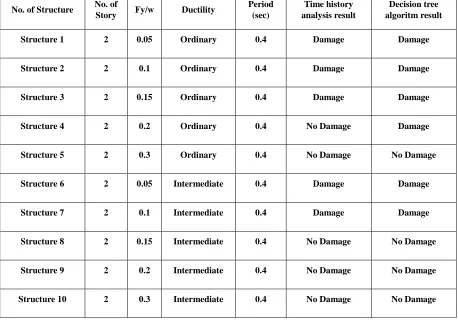
programming [17]. Furthermore, damage values were calculated using the decision trees developed in this article. Temban record with the magnitude (M) of 6.2 and distance (R) of 10.8 km from the site were used to calculate damage in both methods. This earthquake record was applied to 30 buildings with different structural characteristics and number of stories and results of these two methods were compared with each other, as shown in Tables 8-9 and Figs. 8-10. According to the comparison, the obtained results from decision tree algorithm were more acceptable than the time-history analyses.

Table 8. Characteristics of the used buildings and validation of the results based on damage- No damage classes

Decision tree algoritm result Time history

analysis result Period

(sec) Ductility

Fy/w No. of

Story No. of Structure

Damage Damage

0.4 Ordinary

0.05 2

Structure 1

0.1 2

Structure 2

0.15 2

Structure 3

Damage No Damage

0.2 2

Structure 4

No Damage No Damage

0.3 2

Structure 5

0.4 Intermediate

0.05 2

Structure 6

0.1 2

Structure 7

0.15 2

Structure 8

0.2 2

Structure 9

0.3 2

(15)

(16)

Table 9. Characteristics of the buildings used in this study and validation based on three damage classes (repairable, beyond repair, and total collapse)

Decision tree algoritm result Time history

analysis result Period (sec) Ductility Fy/w No. of Story

No. of

Structure Collapse Collapse 0.4 Ordinary 0.05 2 Structure 1 Collapse Collapse 0.4 Ordinary 0.1 2 Structure 2 Collapse Collapse 0.4 Ordinary 0.15 2 Structure 3 Beyond repair - 0.4 Ordinary 0.2 2 Structure 4 Collapse Collapse 0.4 Intermediate 0.05 2 Structure 6 Collapse Collapse 0.4 Intermediate 0.1 2 Structure 7 Collapse Collapse 0.4 Special 0.05 2 Structure 11 Collapse Collapse 0.8 Ordinary 0.05 5 Structure 16 Collapse Collapse 0.8 Ordinary 0.1 5 Structure 17

a b

Figure 8. Comparison results of damage for a 2-story building obtained from a) decision tree algorithm, and b) time-history nonlinear analyses related to the first phase of classification (damage, non-damage)

st 1 st 2 st 3 st 4 st 6 st 7 st 11 Damage st 5 st 8 st 9 st 10 st 12 st 13 st14

st 15 No Damage st 1

st 2 st 3 st 6

st 7 st 11 Damage st 4 st 5 st 8 st 9 st 10 st 12 st 13 st 14 st 15

(17)

a b

Figure 9. Comparison results of damage for a 5-story building obtained from a) decision tree algorithm, and b) time-history nonlinear analyses related to the first phase of classification (damage, non-damage)

a b

Figure 10. Comparison results of damage for a 2-story building obtained from a) decision tree algorithm, and b) time-history nonlinear analyses related to the second phase of classification (repairable, beyond

repair, and total collapse)

st 16

st 17

Damage st 18

st 19 st 20 st 21 st 22 st 23 st 24 st 25 st 26 st 27 st 28 st 29 st 30

No Damage st 16

st 17

Damage st 18

st 19 st 20 st 21 st22

st 23 st 24 st 25 st 26

st 27 st 28 st 29 st 30

No Damage

st 1 st 2 st 3 st 6 st 7 st 11 st 16 st 17

Collapse

st 4 Beyond Repair

Repairable st 1

st 2 st 3 st 6

st 7 st 11 st 16

st 17 Collapse

(18)

9. Conclusion

In this study, decision tree classification algorithm was used to predict damage to steel structures. Input and output parameters required for training and evaluating the decision-making tree algorithm were obtained from the results of damage spectra for steel structures and using Krawinkler damage index. Input parameters for algorithm training included structural characteristics like strength, ductility, and its period. Also, characteristics of earthquake record were magnitude and distance to the site. The output parameter was also in two phases. The first phase indicated damage or no damage conditions of the structure, while the second phase showed damage type. In order to evaluate this approach, results of the damage classification obtained from decision tree algorithm were compared with those obtained from time-history analysis. Accuracy of the applied method in this study was directly related to that of the data used to train the network. Since there are some insignificant and outlier data in teaching damage prediction patterns, such as larger than 1 damage, this article utilized data classification method, which was structural damage in this article. The results were presented as qualitative damage prediction based on tree classification algorithm.

REFERENCES

[1] Riddell, R.Garcia, JE.Garces, E. (2002)."Inelastic deformation response of SDOF systems subjected to earthquakes". Earthquake Eng Struct Dyn, 515,pp.31–38. [2] Karbassi, A. Mohebi, B. Rezaee, S. Lestuzzi, P. (2014). "Damage prediction for regular reinforced concrete buildings using the

decision tree algorithm". Computers and Structures ,130, 46–56.

[3] Amziane, S., Dube, JF.(2008)." Global RC structural damage index based on the assessment of local material damage". J Adv Concr Technol,6,459–68.

[4] Wahalthantri, BL.Thambiratnam, DP. Chan, THT. Fawzia, S.(2012)."An improved method to detect damage using modal strain energy based damage index". Adv Struct Eng,15,727–42.

[5] Benavent-Climent,. A.( 2011)."A seismic index method for vulnerability assessment of existing frames: application to RC structures with wide beams in Spain". Bull Earthquake Eng,9,491–517.

[6] Bozorgnia,Y. Bertero,V.(2003)."Damage Spectra: Characteristics and Applications to SeismicRisk Reduction". Journal of Structural Engineering, 129, no. 10,1330-1340.

[7] Elenas. A. Meskouris, K. (2001)." Correlation study between seismic acceleration parameters and damage indices of structures". Eng Struct,23,698–704.

[8] Ghobarah, A. and Osman, A.( 1995)." Seismic Damage Assesment in Low-Rise Steel Moment Resisting Frames". 10th European Conference on Earthquake Engineering.

[9] DiPasquale, E. Cakmak, AS. (1987)."Detection and assessment of seismic structural damage".State University of New York at Buffalo, National Center for Earthquake Engineering Research.

[10] McCabe, SL.Hall ,WJ. (1989)."Assessment of seismic structural damage". J Struct Eng ASCE 115,2166–2183.

[11] Krawinkler, H. Zohrei, M. (1983)."Cumulative Damage in Steel Structures Subjected to Earthquake Ground Motions. Computers and Structures".,16, 531-541.

[12] Building and Housing Research Center (BHRC), http://www.bhrc.ir/.

[13] Hashemi, S. A. H. Ghodrati Amiri ,G.

Mohebi, B. Hamedi, F.

(19)

relation for damage spectrum in X-braced steel structures with neural network. JVE. Internationalltd".Journal of Vibroengineering , 16, 8. 3879-3900 [14] Witten, IH. Frank, E. Hall, MA.

(2011).,"Data mining: practical machine learning tools andtechniques". 3rd ed. Burlington: Morgan Kaufmann.

[15] Quinlan JR. C4.5: programs for machine learning. Morgan KaufmannPublishers; 1993.

[16] Hall ,M. Frank, E. Holmes, G. Pfahringer, B. Reutemann, P. Witten, IH. The WEKA data mining software: an update. SIGKDD Explor 2009;11(1).

[17] Matlab (7.6.0.324(R2008a)).[The Language of Technical Computing].USA:Math Works, Inc,U.S. patents.