Volume 27 - Article 20 | Pages 543–592

(1)

in the population sciences published by the Max Planck Institute for Demographic Research Konrad-Zuse Str. 1, D-18057 Rostock · GERMANY www.demographic-research.org

DEMOGRAPHIC RESEARCH

VOLUME 27, ARTICLE 20, PAGES 543-592

PUBLISHED 25 OCTOBER 2012

http://www.demographic-research.org/Volumes/Vol27/20/ DOI: 10.4054/DemRes.2012.27.20

Research Article

Smoothing and projecting age-specific

probabilities of death by TOPALS

Joop de Beer

This open-access work is published under the terms of the Creative Commons Attribution NonCommercial License 2.0 Germany, which permits use, reproduction & distribution in any medium for non-commercial purposes, provided the original author(s) and source are given credit.

(2)

1 Introduction 544

2 Methods for smoothing age-specific death probabilities 545

3 Methods for projecting life expectancy 546

4 TOPALS and partial adjustment model 550

5 The use of TOPALS for smoothing age-specific probabilities of death 552

6 Scenarios of age-specific probabilities of death 558

6.1 Baseline scenario 559

6.2 Convergence scenario 565

6.3 Acceleration scenario 567

7 Conclusion and discussion 569

8 Acknowledgements 572

References 573

Appendix A: Death probabilities for Germany, Italy, and Hungary 577

Appendix B: Risk ratios 586

Appendix C: Estimated coefficient of partial adjustment model 588

(3)

Smoothing and projecting age-specific probabilities of death by

TOPALS

Joop de Beer1

Abstract

BACKGROUND

TOPALS is a new relational model for smoothing and projecting age schedules. The model is operationally simple, flexible, and transparent.

OBJECTIVE

This article demonstrates how TOPALS can be used for both smoothing and projecting age-specific mortality for 26 European countries and compares the results of TOPALS with those of other smoothing and projection methods.

METHODS

TOPALS uses a linear spline to describe the ratios between the age-specific death probabilities of a given country and a standard age schedule. For smoothing purposes I use the average of death probabilities over 15 Western European countries as standard, whereas for projection purposes I use an age schedule of ‘best practice’ mortality. A partial adjustment model projects how quickly the death probabilities move in the direction of the best-practice level of mortality.

RESULTS

(4)

increase to 80 years for men and 87 years for women in 2060, whereas the Acceleration scenario projects an increase to 90 and 93 years respectively.

CONCLUSIONS

TOPALS is a useful new tool for demographers for both smoothing age schedules and making scenarios.

1. Introduction

TOPALS (tool for projecting age-specific rates using linear splines) is a new relational model for smoothing age schedules. Even though the method is mathematically simple, the model is capable of fitting quite different age schedules. Because the method is simple, it is a flexible and transparent tool for making forecasts and scenarios. The method can be used for making forecasts by estimating a time series model for the parameters from past data. The method can be used for making scenarios by making assumptions about the future time path of the parameters. De Beer (2011) shows how TOPALS can be used to smooth and project age-specific fertility. This article shows how TOPALS can be used for smoothing and projecting mortality for 26 European countries.

TOPALS uses a linear spline to model the ratios between age-specific probabilities of death and a smooth, standard age schedule. The choice of the standard age schedule depends on the aim for which TOPALS is used. If the aim is to smooth age-specific death probabilities, any smooth age schedule can be used. In this article I use the average age-specific death probabilities of 15 Northern, Western, and Southern European countries as standard. If the aim is to make projections, TOPALS can use ‘best practice’ age-specific death probabilities as standard. TOPALS can be used for making projections of age-specific probabilities by making projections of the values of the risk ratios for selected ages (the so-called knots). If it is assumed that the probabilities of death of a given country will move in the direction of the best-practice values, the risk ratios will move to one. In this article I use a projection of age-specific death probabilities of Japanese women as standard age schedule. This can be considered as best-practice mortality since death probabilities of Japanese women have been the lowest in the world since the early 1980s.

(5)

that the difference between the current value and the target value will decline exponentially. If the partial adjustment model is estimated from past data, TOPALS can be used as a tool to make forecasts. If assumptions about the future time path of the risk ratios are made, TOPALS can be used for making alternative scenarios.

In this article I make one projection based on past trends in each of the 26 European countries separately and two alternative scenarios assuming common trends across European countries. All projections use the same standard age schedule. The scenarios differ by assumptions about the value of the coefficient of the partial adjustment model. The Convergence scenario assumes that the coefficient is equal for all European countries, whereas the Acceleration scenario assumes that the future movement towards the best-practice level will be quicker than in the past.

The second section of this article discusses methods for smoothing age-specific death probabilities. The third section gives a brief overview of the literature about methods for projecting mortality. The fourth section describes TOPALS and the partial adjustment model that is used for projecting the parameters of TOPALS. The fifth section shows how TOPALS can be used for smoothing age-specific probabilities of death. Section six describes the use of TOPALS for making three alternative scenarios for 26 European countries. The final section summarizes and discusses the results.

2. Methods for smoothing age-specific death probabilities

The most commonly used indicator of mortality is the mortality rate. The mortality rate

is the number of deaths at age x divided by the number of person-years at risk at age x.

Mortality rates can be estimated from population statistics based on an assumption

about the exposure time, i.e. an assumption about when deaths occur during each time

interval. The death probability is the probability that a person who has reached age x

will die before reaching age x+1. Age-specific death probabilities can be derived from

mortality rates: for example, assuming a uniform distribution of exposure in x, qx =

mx/(1+½ mx) where qx is the death probability at age x and mx is the mortality rate. For

(6)

One advantage of using death probabilities rather than rates is that probabilities are easy to interpret and can simply be used for forecasting (King and Soneji, 2011). Another advantage is that probabilities rather than rates are used for the calculation of life expectancy using a life table. Thus a projection of death probabilities results in a projection of life expectancy without any additional assumptions. For that reason I use TOPALS to make projections of death probabilities rather than mortality rates, as opposed to, for instance, the Lee-Carter method which projects rates. However, using rates instead of probabilities would hardly have led to different results, since even though the levels differ at the oldest ages, the changes over time show a similar pattern.

For individual countries, age-specific death probabilities show a rather irregular pattern. Therefore, for analysing changes over time and making projections, it is useful to smooth the age pattern. One widely used method to describe the age pattern of mortality across all ages is the Heligman-Pollard model (Heligman and Pollard, 1980). This model includes eight parameters. One problem in using the Heligman-Pollard model for projection purposes is that the individual parameters lack a direct demographic interpretation. Another problem is that the parameter values are interdependent (McNown et al., 1995). Booth (2006) concludes that the Heligman-Pollard model is not very useful for forecasting.

Instead of specifying a model including many parameters one alternative procedure is to estimate a relational model. One chooses a smooth age pattern and specifies a simple model that describes how the age-specific rates to be smoothed differ from the standard age schedule. Brass (1974) developed a relational method based on assuming a linear relationship between the logits of the survivorship probabilities. The intercept and the slope of the linear function can be estimated by OLS regression. The intercept is related to the life expectancy at birth (Brass, 1974). Brass suggests projecting the intercept and the slope on the basis of past trends. One problem, however, is that if death rates across time are related to the same standard age schedule the fit of the model tends not to be accurate in all years. In that case, changes in the intercept and slope do not accurately describe changes in the age pattern of mortality. Since TOPALS is less sensitive to the choice of the standard age schedule, it is better capable of describing and projecting changes over time.

3. Methods for projecting life expectancy

(7)

86 years in 2045 (Fries, 1989). Since life expectancy of Japanese women has reached that level in 2008 already, Fries’ estimate clearly is too low. Oeppen and Vaupel (2002) argue that there is no sign of a slowing down in the increase in life expectancy. In contrast, they note that the ‘best practice’ life expectancy has been increasing linearly by 2.5 years per decade during the past 150 years. They expect that this trend will continue in the coming decades. Vallin and Meslé (2009) show that the straight line of Oeppen and Vaupel consists of several segments with different slopes. They show that the slope has declined from .32 in the period 1886-1960 to .23 in the period 1960-2005. Even though their estimate of the slope for the most recent period is close to Oeppen and Vaupel’s estimate for the longer period, their estimates show that there has not been a constant increase during 150 years as suggested by Oeppen and Vaupel. Thus it may be less obvious that this trend will continue in the long run as claimed by Oeppen and Vaupel. In a recent article, Torri and Vaupel (2012) acknowledge that the trend may have changed and they estimate the increase in life expectancy since 1900 rather than 1840. However, they ignore the slowing down of the increase since 1960 shown by Vallin and Meslé.

Since 1981, Japanese women have had the highest life expectancy at birth. Figure 1 shows that, during that period, the development of life expectancy at birth of Japanese women is close to linear. Thus one may project life expectancy at birth of Japanese women by a random walk model with drift:

c e e

E( 0,t )= o,t−1 + (1)

where e0,t = life expectancy at birth in year t and c is a constant term (‘drift’). In 2008,

life expectancy of Japanese women equaled 86 years. For the period 1978-2008, the

estimate of c equals 0.26. This corresponds with Oeppen and Vaupel’s estimate. Note

that Oeppen and Vaupel use a much longer time series of best-practice life expectancies. Before Japan, countries such as Sweden, Denmark, and New Zealand contributed to the time series of maximum life expectancy.

(8)

Figure 1: Life expectancy at birth of Japanese women, 1950-2100

50 60 70 80 90 100 110 120

1950 1970 1990 2010 2030 2050 2070 2090

ye

ar

s

Solid line: observed values, 1950-2008; dotted line: random walk with drift (fitted values, 1978-2008; projected values, 2009-2100); dashed line: Lee-Carter model (projected values 2009-2100).

Even though Bongaarts (2006) agrees that life expectancy will continue to increase, he assumes that the future increase will be lower than in the past. He argues that the strong decline in death rates at young ages observed in the last 50 years cannot continue since the death probabilities have already reached very low levels. Likewise Olshansky and Carnes (1994) argue that a linear projection of life expectancy is very optimistic as this can only be achieved if the decline in age-specific probabilities of death will accelerate. Olshansky et al. (2005) and Stewart, Cutler, and Rosen (2009) argue that an increase in obesity may reduce the increase in life expectancy in future.

(9)

expectancy will continue to increase linearly in the future. Moreover life expectancy in individual countries has not shown a linear increase over very long periods (Lee, 2006). Thus, rather than projecting future life expectancy at birth based on the extrapolation of a time series of life expectancy, it seems useful to project time series of the underlying age-specific probabilities of death. The Lee-Carter method has become the most widely applied model for making projections of age-specific mortality rates (Booth, 2006). Lee and Carter (1992) decompose the level of mortality rates into age-dependent and time-age-dependent components:

. (2)

t x x t

x a bk

m

E(ln ,)= +

where mx,t is the mortality rate at age x in year t, ax describes the average age pattern, kt

describes the change in mortality rates over time, and bx determines how the change

varies by age. Lee and Carter (1992) assume that

_∑

=

_∑

=

x x

b 1 and

t t

k 0 . These

normalizations make it possible to obtain unique least squares estimates of the values of

ax, bx, and kt. Since ax and bx are time invariant, future values of mx,t can be projected by

projecting kt. In almost all applications, kt is projected by a random walk with drift

model (Booth, 2006). This implies that, for each age x, the projected change in the

mortality rate is exponential.

Applying the Lee-Carter model to the time series of mortality rates of Japanese women for the period 1978-2008 leads to a projection of life expectancy at birth in 2060 of 97.6 years and a value of 103.0 years in 2100. Figure 1 shows that, in the long run, the projections of the Lee-Carter model are lower than those of linear projections of the time series of life expectancy. The reason is that the Lee-Carter model projects an exponential decline in mortality rates which implies that as mortality rates become low, the decline will slow down.

Several authors have proposed variants of the Lee-Carter method. Shang, Booth, and Hyndman (2011) examine the forecast accuracy of nine variants and extensions of the Lee-Carter method. They conclude that several variants outperform the Lee-Carter model for one-year-ahead forecasts, but that the Lee-Carter model performs well for ten-years-ahead projections. They did not examine longer forecast intervals.

(10)

4. TOPALS and partial adjustment model

TOPALS describes the ratios of the age-specific probabilities of death of a given country and those according to a standard age schedule by a linear spline, which is a piecewise linear curve. If the standard age schedule shows a smooth pattern, multiplying the linear spline by the standard age schedule will produce a smooth age

pattern of the death. The model for the age schedule at time t = 0 is:

x x x rQ

q = (3)

where qx is the observed probability of death at age x, rx is the risk ratio, and Qxis the

probability of death according to the standard age schedule. The age pattern of the risk ratios can be described by the linear spline function:

∑

(4)

= −

+

= n

j j j xj

x a b x k D

r

1

) (

where Dxj= 0 if x≤ kj and Dxj= 1 otherwise, kj are the knots (i.e., the ages at which the

successive linear segments are connected), and a and bj are the parameters to be

estimated. The knots can be chosen in such a way that the fit of the linear spline to the data is optimal (e.g., by applying a non-linear least squares method). However, this would result in different knots for different countries. Since I want to make

cross-country comparisons, I decided to fix the location of the knots a priori at the same ages

for each country: at ages 20, 30, 40, …, 100, 109. Since age-specific probabilities of death for ages 0-20 show an irregular pattern, I assume that the risk ratios for these ages are equal: r0 = r1 = …. = r20. They are calculated as the ratio of the average of (q0...q20)

and the average of (Q0…Q20). This implies that the slope of the spline is assumed to

equal zero for ages 0-20. The values of a and bj are determined in such a way that the

values of the spline at the knots equal the observed values (De Beer, 2011).

In general a quadratic or cubic spline produces a smoother curve than a linear spline. However, since the linear spline is fitted to the relative risks rather than to the probabilities of death, a linear spline is sufficient to produce a smooth age schedule for the probabilities of death as long as the standard age schedule is smooth. One benefit of using a linear spline is that it is much easier to interpret than a cubic spline.

Projections of probabilities of death can be made by the time series model:

x t x t

x r Q

(11)

Thus projections of age-specific death probabilities require assumptions about the model age schedule and about the time path of the risk ratios. For making projections I use the age schedule of a ‘best practice’ country as standard. This implies that the risk ratios indicate to what extent probabilities of death in a given country are higher than the target level. If one assumes that probabilities of death will decline, they will move in the direction of the best-practice level and the risk ratios will thus move towards a value of 1. For that reason I use a partial adjustment model for projecting the risk ratios, assuming that the risk ratios will move towards 1:

) 1 ( 1 )

(rx,t = + x rx,t−1−

E ϕ (6)

where 0 ≤φx≤ 1. This model assumes that the value of rx,t is closer to 1 than the value

in the previous year. The lower the value of φx, the quicker rx,t will move towards 1. If

φx = 1 model (6) describes a random walk, and thus rx,t will not converge to 1. If the

probabilities of death are higher than those according to the standard schedule, (6) implies that the death probabilities are projected to decrease whereas, if the death probabilities are smaller than those according to the standard schedule, the model

projects an increase. It would be possible to assume that φx may exceed 1. However,

that would imply that death probabilities would continue to increase. This does not seem a plausible assumption in the long run.

The partial adjustment model (6) resembles the geometric mean-reverting process model used by Torri and Vaupel (2012) to project how the gap between life expectancy of a given country and the best-practice life expectancy will decline. The main two differences are that they apply the model to life expectancy rather than to death probabilities and that their model includes a long-run equilibrium level of the gap. They assume that the gap will not reduce to zero but to some positive value, whereas model (6) implies that the life expectancy of each country will move towards the target level though it may take very long before this level will be reached.

The partial adjustment model assumes that there is a target level towards which death probabilities will decline. However, TOPALS can be used to make projections using other models as well. For example, one can project the risk ratios at the knots by using a random walk with drift model for the logarithms of the risk ratios:

t c r r

E(ln _x,_t)=ln _x,0+ _x . (7)

(12)

t c r Q q

E(ln x,t)=ln x+ln x,0+ x (8)

This model is similar to the Lee-Carter model. Both models project a linear change of the logarithms of the probabilities of death. However, the projections are not exactly the same for two reasons. First, using TOPALS the random walk model is used for projecting probabilities of death at the knots only and the projections for ages in between are obtained from the linear spline of risk ratios (4). This provides a smooth

age pattern for qx,t, whereas the Lee-Carter projects an irregular pattern. Note that

several authors suggest to smooth the mortality rates or the age-specific components of the Lee-Carter model to obtain smooth projections (e.g., Renshaw and Haberman, 2003; Hyndman and Ullah, 2007). Secondly, the drift in (8) is estimated from the time series

lnqx,t for each knot, whereas in applying the Lee-Carter model the drift is estimated

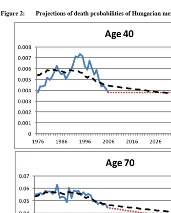
from the time series kt, i.e. the drift is the same for all ages. Figure 2 illustrates the

difference between both projections of death probabilities. The figure shows projections of the death probability of Hungarian men at ages 40 and 70. The observation period is 1976-2006. The dotted lines show the projections that are based on TOPALS using the random walk with drift model. The dashed lines show the Lee-Carter projections. The latter projections extrapolate the fitted time series rather than the observed time series.

5. The use of TOPALS for smoothing age-specific probabilities of

death

(13)

Figure 2: Projections of death probabilities of Hungarian men, ages 40 and 70

0 0.001 0.002 0.003 0.004 0.005 0.006 0.007 0.008

1976 1986 1996 2006 2016 2026 2036 2046

Age

40

0 0.01 0.02 0.03 0.04 0.05 0.06 0.07

1976 1986 1996 2006 2016 2026 2036 2046

Age

70

(14)

For Germany, the Human Mortality Database includes time series starting in 1990. For previous years the database includes time series for both West and East Germany. I estimated time series for Germany prior to 1990 by calculating the weighted average of death probabilities of West and East Germany using population size as weights. Since West Germany includes about 80 percent of the total population of Germany, the death probabilities of Germany resemble those of West Germany, but are slightly higher since the East German death probabilities are higher, particularly for men.

The mortality rates included in the Human Mortality Database are smoothed at the highest ages using a logistic model (Wilmoth et al., 2007) following Thatcher’s suggestion (Thatcher, 1999). It is assumed that the death probability at age 110 equals 1 across all countries. As a consequence, the age patterns at the oldest ages look similar across countries.

I specified a standard age schedule by calculating the weighted average of the age-specific death probabilities for men and women of 15 Northern, Western, and Southern European countries: Austria, Belgium, Denmark, Finland, France, Germany, Ireland, Italy, Netherlands, Norway, Portugal, Spain, Sweden, Switzerland, and the United Kingdom. The other 12 countries were excluded as they have a strongly different mortality pattern. Each of the selected 15 countries has a life expectancy of men of 75 years or higher and a life expectancy of women of 80 years or higher. The range between the minimum and maximum life expectancies across these 15 countries is relatively small compared with the other 12 countries. I weighted the death probabilities by total population size for men and women separately. I label this as the NWS European average. Since there are some irregular fluctuations at ages below 20 and at older ages, I applied TOPALS to smooth the age curve, using the Heligman-Pollard model as the standard age schedule. Figure 3 shows the logarithms of the average age-specific death probabilities for women.

(15)

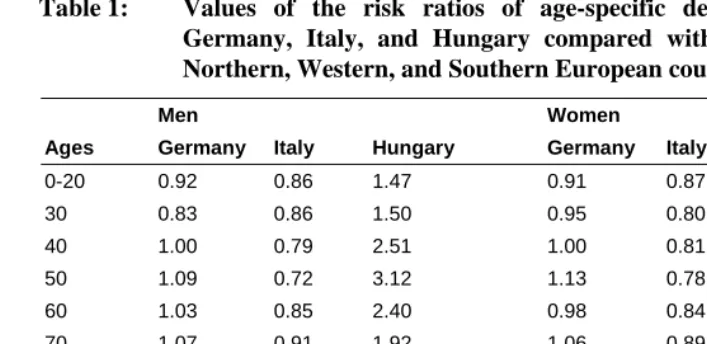
high mortality between ages 40 and 60. The death probabilities around age 50 are three times as high as the NWS European average. At older ages the differences are considerably smaller. This pattern is typical for most Eastern European countries, especially for men (see Tables B.1 and B.2 in Appendix B). Note that for most countries the risk ratios at the oldest ages are close to 1. This is caused by the fact that in the Human Mortality Database the age-specific mortality rates at old ages are smoothed using the same method across countries.

Figure 3: Age-specific death probabilities, women, weighted average of 15 Northern, Western, and Southern European countries, 2006

0.00001 0.0001 0.001 0.01 0.1 1

0 5 10 15 20 25 30 35 40 45 50 55 60 65 70 75 80 85 90 95 100105

(16)

Table 1: Values of the risk ratios of age-specific death probabilities of Germany, Italy, and Hungary compared with the average of 15 Northern, Western, and Southern European countries, 2006

Men Women

Ages Germany Italy Hungary Germany Italy Hungary

0-20 0.92 0.86 1.47 0.91 0.87 1.25

30 0.83 0.86 1.50 0.95 0.80 1.60

40 1.00 0.79 2.51 1.00 0.81 2.07

50 1.09 0.72 3.12 1.13 0.78 2.19

60 1.03 0.85 2.40 0.98 0.84 1.85

70 1.07 0.91 1.92 1.06 0.89 1.86

80 1.01 0.96 1.46 1.08 0.89 1.60

90 1.06 0.98 0.87 1.12 0.97 1.14

100 1.09 0.99 0.86 1.11 0.98 1.01

109 1.04 0.98 0.81 1.04 0.98 0.94

(17)

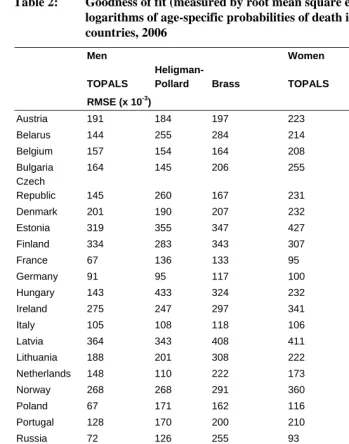
Table 2: Goodness of fit (measured by root mean square error, RMSE) of the logarithms of age-specific probabilities of death in 26 European countries, 2006

Men Women

TOPALS

Heligman-Pollard Brass TOPALS

Heligman-Pollard Brass

RMSE (x 10-3)

Austria 191 184 197 223 255 232

Belarus 144 255 284 214 192 249

Belgium 157 154 164 208 248 218

Bulgaria 164 145 206 255 184 353

Czech

Republic 145 260 167 231 244 229

Denmark 201 190 207 232 234 271

Estonia 319 355 347 427 418 417

Finland 334 283 343 307 319 296

France 67 136 133 95 212 135

Germany 91 95 117 100 176 132

Hungary 143 433 324 232 327 302

Ireland 275 247 297 341 306 330

Italy 105 108 118 106 172 112

Latvia 364 343 408 411 369 419

Lithuania 188 201 308 222 222 265

Netherlands 148 110 222 173 192 184

Norway 268 268 291 360 362 350

Poland 67 171 162 116 170 159

Portugal 128 170 200 210 214 247

Russia 72 126 255 93 88 246

Slovakia 232 236 246 262 235 322

Spain 129 131 130 106 214 142

Sweden 188 292 221 228 298 229

Switzerland 196 217 214 274 299 282

Ukraine 126 102 251 122 92 253

United

Kingdom 76 91 94 90 116 117

(18)

One benefit of using TOPALS rather than the Brass relational model is that TOPALS is less sensitive to the choice of the standard age schedule. In the next section I will use projected age-specific death probabilities of Japanese women as a standard age schedule for making projections of the death probabilities for European countries. The Japanese age pattern differs quite strongly from the European schedule. The Japanese age-specific death probabilities at older ages are considerably lower than the European. If this age schedule is used as standard for fitting TOPALS the RMSE increases only slightly compared with that shown in Table 2. However, if this age schedule is used as standard for fitting the Brass relation model the fit of the Brass model becomes very poor. Thus the Brass model is much more sensitive to the choice of the standard age schedule than TOPALS.

6. Scenarios of age-specific probabilities of death

Rather than making one forecast of the most probable future development of death probabilities, I used TOPALS to make three alternative scenarios. For each scenario I use the same ‘target’ age-specific probabilities of death, viz. projected age-specific probabilities of death of Japanese women. Figure 4 shows the age-specific death probabilities of Japanese women in 2008 and compares these with the NWS European average. In section 3 I showed that if one assumes that life expectancy at birth of Japanese women will continue to increase linearly in the next 50 years, it will reach a level of 99.6 years in 2060 (see Figure 1). This corresponds with a reduction of all age-specific probabilities of death by 74%. Because this produces a rather irregular age pattern, I used TOPALS to smooth the age pattern, with the NWS European average as standard age curve. The dashed line in Figure 4 shows the smooth target pattern. Note that the age pattern of death probabilities of Japanese women differs from the NWS European average. Around age 70 the differences are larger than around age 40 or age 90. As a consequence, assuming the same percentage decrease across all ages for Japanese women produces a target pattern that implies different rates of change for European women.

For the ages at the knots I made time series of risk ratios by dividing the death probabilities for each country by the target values. The rate of decline in the risk ratios differs across ages, sexes, and countries. For example, for German and Italian men, the decline at age 50 has been larger than at age 90 (see Figure A.4 in Appendix A). In contrast, the risk ratio increased for Hungarian men at middle ages until the 1990s and even though there has been a decrease since, the level is still very high. For women, the differences across ages are considerably smaller than for men.

(19)

call this the Baseline scenario. The second scenario assumes that the values of φ are equal for all countries. This scenario assumes that there will be a similar trend across European countries. I call this the Convergence scenario. The third scenario assumes that the future decrease in death probabilities will exceed that in the last three decades. I label this the Acceleration scenario.

Figure 4: Age-specific death probabilities: Japanese women, 2008; average of Northern, Western, and Southern European countries, 2008; and target pattern for 2060

0.00001 0.0001 0.001 0.01 0.1 1

0 10 20 30 40 50 60 70 80 90 100

age

Solid line: Japanese women in 2008; dotted line: average of 15 Northern, Western, and Southern European countries in 2006; dashed line: target values (Japanese women in 2060)

6.1 Baseline scenario

The Baseline scenario can be considered an extrapolation of the past trends in the risk

ratios for each country. I estimate the parameter φx of the partial adjustment model (6)

(20)

by Lee and Miller (2001). First, the development of mortality of men in most European countries has been more stable since the 1970s than since 1950. Second, this estimation period is similar to the period that Eurostat chooses as basis for their latest scenarios (Lanzieri, 2009). Eurostat selected the fitting period 1977-2005 on the basis of goodness of fit according to the method proposed by Booth et al. (2002). Below I will discuss the effect of the choice of the base period on the projections.

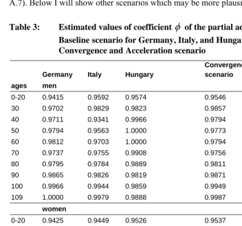
The values of φ determine how strongly the observed probabilities of death move

towards the target levels. Table 3 shows the estimated values of φfor Germany, Italy,

and Hungary. If φ is close to 1, the projections will move very slowly to the target

value, and thus death probabilities will decline slowly. If φ equals 1, the projected value

equals the last observed value and does not move towards the target level. This is the

case for Hungarian men at ages 50 and 60. For Italy, the values of φ for most ages are

lower than for the other two countries. Thus, the model will project a more rapid

decline of death probabilities for Italy. The estimated values of φ for older ages tend to

be closer to 1 than for younger ages (Appendix C shows the estimated values of φ for

all countries in this study). The explanation is that there has been a slow decrease in death probabilities at older ages. This implies that the Baseline scenario projects only limited decrease at older ages in the future. Note that, even though I assume the same target levels of probabilities of death across all countries and for both sexes, this does not imply that this is a convergence scenario. The projections differ across countries for two reasons: the gap between the current death probabilities and the target values differ as well as the values of φ.

By multiplying the projected risk ratios by the target values of the probabilities of death, I obtain projections of the death probabilities for each country. Generally the projected rates of change are similar to those according to the Lee-Carter model (see Figures A.5, A.6 and A.7 in Appendix A which show the projections for ages 50 and 90 for Germany, Italy and Hungary respectively). However in some cases the jump-off value of the Lee-Carter projections differs from the last point in the observation period, which results in differences in the levels of the projections. For example, the projections for Hungarian men aged 90 years, according to the Baseline scenario, are lower than those according to the Lee-Carter model as they start from a lower level (see Figure A.7). The explanation is that the Lee-Carter projections start from the last estimated value of the death probability rather than from the last observed value. I discussed this issue at the end of section 4 (see Figure 3). For this reason Lee and Miller (2001) suggest to use the last observed value as jump-off value for the projections of the Lee-Carter model. This would make the Lee-Lee-Carter projections closer to the Baseline scenario.

(21)

(see Figure A.8 in Appendix A which compares the age-specific death probabilities for Germany, Italy, and Hungary projected by the Baseline scenario with the pattern in the last observation year and with the target pattern). This reflects the relatively strong decline in death probabilities at young ages and the slow decline at older ages during the observation period. For Hungarian men, the Baseline scenario does not project a decrease of death probabilities at middle ages because of the unfavorable trend during the estimation period. One may question whether this is a plausible scenario since recent years have shown a decrease in death probabilities at middle ages (see Figure A.7). Below I will show other scenarios which may be more plausible.

Table 3: Estimated values of coefficient

φ

of the partial adjustment model, Baseline scenario for Germany, Italy, and Hungary with the Convergence and Acceleration scenario

Germany Italy Hungary

Convergence scenario

Acceleration scenario ages men

0-20 0.9415 0.9592 0.9574 0.9546 0.9116

30 0.9702 0.9829 0.9823 0.9857 0.9715

40 0.9711 0.9341 0.9966 0.9794 0.9588

50 0.9794 0.9563 1.0000 0.9773 0.9548

60 0.9812 0.9703 1.0000 0.9794 0.9642

70 0.9737 0.9755 0.9908 0.9756 0.9517

80 0.9795 0.9784 0.9889 0.9811 0.9622

90 0.9865 0.9826 0.9819 0.9871 0.9747

100 0.9966 0.9944 0.9859 0.9949 0.9899

109 1.0000 0.9979 0.9888 0.9987 0.9974

women

0-20 0.9425 0.9449 0.9526 0.9537 0.9057

30 0.9748 0.9730 0.9745 0.9817 0.9642

40 0.9689 0.9707 0.9815 0.9790 0.9576

50 0.9777 0.9671 0.9961 0.9755 0.9517

60 0.9769 0.9685 0.9905 0.9781 0.9563

70 0.9702 0.9715 0.9863 0.9734 0.9481

80 0.9746 0.9715 0.9853 0.9749 0.9499

90 0.9834 0.9804 0.9828 0.9829 0.9659

(22)

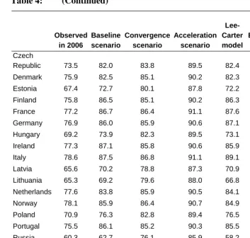
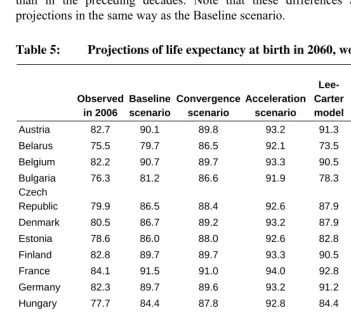
Tables 4 and 5 show the values of life expectancy at birth in 2060 for men and women respectively which result from the projections of the age-specific death probabilities according to the Baseline scenario. This scenario projects that life expectancy at birth in 2060 for men in Northern, Western, and Southern European countries will range from 83 to 88 years (Table 4) and for women from 87 to 92 years (Table 5). For Central and Eastern European countries the range is wider: from 63 to 82 years for men and from 76 to 87 years for women. This is due to the fact that the development of death probabilities in countries such as Belarus, Ukraine, and Russia has been much worse than in countries such as Czech Republic, Slovakia, and Poland. On average, the Baseline scenario is slightly higher than the Eurostat scenario EUROPOP2008 for Northern, Western, and Southern European countries. For Central and Eastern European countries the Eurostat scenario is much higher as Eurostat assumes strong convergence towards the low levels in Northern, Western, and Southern Europe.

Tables 4 and 5 show the Lee-Carter projections as well. For most Northern, Western, and Southern European countries, the differences between the Baseline scenario and the Lee-Carter projection are moderate. For the 15 Northern, Western, and Southern European countries, half of the projections of the Baseline scenario are higher than the Lee-Carter projections and vice versa. For the Central and Eastern European countries, the Baseline scenarios are higher. One explanation is that recent improvements in mortality in these countries have a larger effect on the Baseline scenario as the jump-off value is lower than for the Lee-Carter method, as discussed above. Moreover, the projections based on the partial adjustment projections are

restricted by the assumption that φ≤ 1. Thus, if, at certain ages, death probabilities have

increased in the observation period, the model projects a constant future level. In contrast, the projections of the Lee-Carter model project an increase in death probabilities at those ages.

Table 4: Projections of life expectancy at birth in 2060, men

Observed in 2006

Baseline scenario

Acceleration scenario

Lee- Carter model

EUROPOP 2008

Linear projection

life expectancy

Austria 77.1 86.6 86.2 90.7 87.7 84.9 93.1

Belarus 63.6 67.9 78.3 86.9 59.7 n.a. 57.6

Belgium 76.5 86.6 85.6 90.4 85.9 84.4 90.3

(23)

Table 4: (Continued)

EUROPOP 2008

Czech

Republic 73.5 82.0 83.8 89.5 82.4 83.2 85.0

Denmark 75.9 82.5 85.1 90.2 82.3 84.3 84.9

Estonia 67.4 72.7 80.1 87.8 72.2 80.8 72.5

Finland 75.8 86.5 85.1 90.2 86.3 84.3 90.7

France 77.2 86.7 86.4 91.1 87.6 85.1 91.6

Germany 76.9 86.0 85.9 90.6 87.1 84.9 92.8

Hungary 69.2 73.9 82.3 89.5 73.1 81.9 73.6

Ireland 77.3 87.1 85.8 90.6 85.9 85.2 91.5

Italy 78.6 87.5 86.8 91.1 89.1 85.5 94.4

Latvia 65.6 70.2 78.8 87.3 70.9 80.5 68.6

Lithuania 65.3 69.2 79.6 88.0 66.8 80.4 63.5

Netherlands 77.6 83.8 85.9 90.5 84.1 84.9 88.6

Norway 78.1 85.9 86.4 90.7 84.9 85.2 89.2

Poland 70.9 76.3 82.8 89.4 76.5 82.5 78.2

Portugal 75.5 86.1 85.2 90.3 85.5 84.1 93.5

Russia 60.3 62.7 76.1 85.9 58.2 n.a. 57.0

Slovakia 70.4 74.8 82.1 88.9 74.5 82.0 76.5

Spain 77.6 85.9 86.4 91.0 86.0 84.9 89.9

Sweden 78.7 85.8 86.5 90.8 86.0 85.4 90.4

Switzerland 79.1 87.8 87.2 91.3 87.8 85.8 92.5

Ukraine 62.3 64.6 77.3 86.5 58.5 n.a. 56.2

United

Kingdom 77.2 86.2 86.2 90.9 86.8 85.0 91.0

(24)

been 10 years longer, projections of life expectancy for the year 2060 would have been about two years lower for Germany and Italy. If the period would have been 10 years shorter, the projections for Hungary would have been three years higher. These differences can be explained by different developments in mortality across countries. The relatively low life expectancy projected on the basis of the longer estimation period for Germany and Italy is due to the relatively poor development of mortality in the 1960s. The relatively high projection for Hungary based on the short estimation period can be explained by the fact that the recent development of mortality is more favorable than in the preceding decades. Note that these differences affect the Lee-Carter projections in the same way as the Baseline scenario.

Table 5: Projections of life expectancy at birth in 2060, women

EUROPOP 2008

Austria 82.7 90.1 89.8 93.2 91.3 89.2 96.3

Belarus 75.5 79.7 86.5 92.1 73.5 n.a. 74.1

Belgium 82.2 90.7 89.7 93.3 90.5 88.9 94.3

Bulgaria 76.3 81.2 86.6 91.9 78.3 86.5 80.6

Czech

Republic 79.9 86.5 88.4 92.6 87.9 87.8 90.1

Denmark 80.5 86.7 89.2 93.2 87.9 88.4 87.4

Estonia 78.6 86.0 88.0 92.6 82.8 87.5 86.1

Finland 82.8 89.7 89.7 93.3 90.5 89.3 94.5

France 84.1 91.5 91.0 94.0 92.8 90.1 96.6

Germany 82.3 89.7 89.6 93.2 91.2 89.1 95.2

Hungary 77.7 84.4 87.8 92.8 84.4 87.3 86.7

Ireland 81.9 90.5 89.8 93.4 90.2 89.2 95.2

Italy 84.1 91.4 90.6 93.7 93.8 90.0 98.2

Latvia 76.5 82.0 86.7 92.0 79.9 86.8 80.4

Lithuania 77.1 82.0 87.1 92.2 78.0 86.9 79.2

Netherlands 81.9 87.4 89.4 93.1 86.7 88.9 89.1

Norway 82.7 88.6 89.8 93.2 89.3 89.2 90.8

Poland 79.6 85.5 88.5 92.9 85.6 88.0 88.5

Portugal 82.2 90.5 89.4 93.1 91.0 88.8 99.3

(25)

Table 5: (Continued)

EUROPOP 2008

Slovakia 78.4 85.3 87.9 92.6 84.5 87.4 86.2

Spain 84.1 91.0 90.5 93.6 92.0 89.6 97.4

Sweden 82.9 89.2 90.0 93.4 88.9 89.3 91.8

Switzerland 84.0 91.6 90.7 93.7 91.1 89.9 94.4

Ukraine 73.8 78.0 85.5 91.5 71.8 n.a. 73.0

United

Kingdom 81.5 89.0 89.6 93.4 88.9 88.9 92.1

6.2 Convergence scenario

There is ample empirical evidence that there has been a converging tendency in mortality declines during the last decades (Wilson, 2001; White, 2002; Janssen et al., 2004; Bongaarts, 2006; Lanzieri, 2009). Life expectancy has increased more strongly in countries that had relatively low life expectancies. In contrast, Moser et al. (2005) find a diverging trend in life expectancy at the worldwide level in the 1990s, which can be explained by unfavorable developments in sub-Saharan Africa due to the HIV/AIDS epidemic and increasing mortality rates at middle ages in Central and Eastern Europe. However, the most recent data examined by Moser et al. refer to 1995-2000. More recent data show that since the mid 1990s death probabilities in Central and Eastern Europe have declined (see, for example, the developments in Hungary shown in figure A.4). Similar developments can be observed in other Central and Eastern countries as well.

(26)

In specifying the Convergence scenario I follow a different approach than Eurostat. I follow the recommendation by Janssen and Kunst (2007) that the average mortality change among similar countries should be used as the basis for the long-run projection of the mortality levels for the individual countries rather than assuming that mortality rates of different countries will reach the same target level by the end of the projection period. One reason is that, as Bongaarts (2006) argues, the average pace of mortality decline across a number of countries reflects the effects of improvements in medical technology and behaviour whereas country-specific deviations are unpredictable. Tuljapurkar et al. (2000) found that the time-dependent parameter of the Lee-Carter model follows a common pattern for the G7 countries. Li and Lee (2005) argue that long-run forecasts for individual countries can be improved by estimating the time-dependent parameter in the Lee-Carter model for a group of countries. Thus there are two reasons for specifying a Convergence scenario. One reason is that one may assume that there is a converging tendency among European countries. However, another important reason is that estimating a common long-run trend for a group of countries may provide a more reliable basis for long-run projections as it excludes the effect of temporary deviations in individual countries. I will come back to this.

I specified a Convergence scenario by estimating the values of φ for time series of

the average probabilities of death of 15 Northern, Western, and Southern European countries. I did not include the Central and Eastern European countries in the estimation of the common parameter as these have followed a different development in the sample

period. The estimated values of φ are given in Table 3. I use these estimated values of φ

for making projections for all European countries including the Central and Eastern European countries.

(27)

As mentioned above, one reason for specifying the Convergence scenario is that one may assume that the estimation of the trend based on average death probabilities over a number of countries is more stable than for separate countries. Thus one would expect that the projections of the Convergence scenario are less sensitive to the choice of the estimation period than those of the Baseline scenario. Appendix D compares the projections of the Convergence scenario based on different estimation periods. The results confirm that the differences between the projections of the Convergence scenario based on different estimation periods are smaller than for the Baseline scenario.

6.3 Acceleration scenario

Even though mortality has declined steadily for a long period, the causes of this decline have changed over time. In the past the main cause of the increase in life expectancy at birth was a decline in infant mortality. This was mainly caused by advances in hygiene, medicine and improvement of living conditions. In the first half of the twentieth century the main causes of death were infectious diseases. In the second half of the century cardiovascular diseases and cancer have become the main causes of death. In recent years mortality by cardiovascular diseases has decreased as a consequence of advances in prevention and treatment in many countries whereas mortality from lung cancer has been falling due to a decline in smoking.

As the causes of changes in death probabilities have altered over time there is no a

priori reason why the decline of mortality in the future should be the same as in the past. Olshansky et al. (2009) assume that in the next fifty years the risk of death may be influenced by accelerated advances in biomedical technology, by changes in behavioural risk factors, and by aggressive management of symptoms. As a consequence, future mortality may decrease more strongly than in the past. In order to take this possibility into account, I developed a third scenario assuming that the future rate of decline in mortality will be stronger than during the observation period.

In the Acceleration scenario I assume that the half time (i.e., the time needed to reach a 50 percent reduction in the difference between the current age-specific probabilities of death and the target values) will be half of that according to the

Convergence scenario. This implies that I assume that the values of φare lower than in

the Convergence scenario. This is illustrated in Figure 5 which shows the projection of the risk ratios for men aged 50 according to the Convergence scenario. The estimated

value of φ equals 0.977. Starting from a risk ratio of 9.12 in 2006, this value of φ

(28)

(corresponding with the year 2021) requires that the value of φ be reduced to 0.955. The

latter value is used for the calculation of the Acceleration scenario. The values of φx for

the ages at the knots for the Acceleration scenario are shown in Table 3.

Figure 5: Values of risk ratio for Convergence and Acceleration scenarios, men aged 50 years, average of Northern, Western, and Southern European countries

1.0 2.0 3.0 4.0 5.0 6.0 7.0 8.0 9.0 10.0

2006 2012 2018 2024 2030 2036 2042 2048 2054 2060 2066

Solid line: Convergence scenario; dashed line: Acceleration scenario.

Tables 4 and 5 show that life expectancy of men in Northern, Western, and Southern European countries will range from 90 to 91 years and for women from 93 to 94 years in 2060 according to the Acceleration scenario. For Central and Eastern Europe, life expectancy will range from 86 to 89 years for men and from 91 to 93 years for women. The gender gap will be approximately three years. For two thirds of the Northern, Western, and Southern European countries this scenario is lower than the linear projection of life expectancy. This illustrates that a linear increase in life expectancy can only be achieved by an acceleration in the decrease of age-specific death probabilities.

(29)

of the other two scenarios). The reason is that the values of φ for ages 80 and over (shown in Table 3) are closer to 1 than the values for middle ages. Olshansky et al. (2009) specify one scenario in which they assume that the slope of the mortality age schedule will be reduced. Using TOPALS, such a scenario can be calculated by

assuming lower values of φ for older ages. For example, one could assume that the

values of φ for ages 80 and over are equal to those for ages 50 to 70. Such a scenario

would lead to an additional increase in life expectancy of 3 to 4 years compared with the Acceleration scenario.

7. Conclusion and discussion

TOPALS is a relational model that can be used to smooth and project age-specific probabilities of death. The method is easy to use, transparent, and flexible while its performance is comparable with that of more complex methods. TOPALS uses a linear spline to model the ratios between age-specific rates of probabilities of a given country and a smooth, standard age schedule. The use of a spline makes TOPALS flexible: it can describe different types of age schedules. De Beer (2011) shows how TOPALS can be used to smooth and project age-specific fertility rates. This article uses TOPALS to smooth age-specific probabilities of death for 26 European countries. Using the average of 15 Northern, Western, and Southern European countries as standard schedule, TOPALS turns out to produce smooth age curves for all European countries. On average, the goodness of fit of TOPALS is better than that of the Heligman-Pollard model and the Brass relational model.

TOPALS can be used to make different types of scenarios. If the standard age schedule describes the best-practice level of mortality, the time series of risk ratios show how strongly death probabilities at different ages in a given country move in the direction of the best-practice levels. In this article I use an extrapolation of age-specific death probabilities of Japanese women as a target age schedule. A partial adjustment

model is used to project the death probabilities at the knots. Instead of a priori

assuming that the target level will be reached before a given forecast horizon, I estimate

the values of the parameter φx of the partial adjustment model which determine how

rapidly death probabilities move towards the target values. The values of φx can be

estimated for each country separately. This produces the Baseline scenario. This scenario turns out to be close to the widely-applied Lee-Carter model. But TOPALS can be used to make alternative scenarios as well.

(30)

countries. The Convergence scenario is based on estimates of the values of φx for

average death probabilities across 15 Northern, Western, and Southern European countries. This scenario projects a narrow range of minimum and maximum life expectancies among the 26 European countries in 2060: 8 years for men and 4 years for women. This is about half of the current range.

An alternative scenario is to assume that, in the future, death probabilities will move more quickly to the target values than they have done during the last decades. The Acceleration scenario assumes that the half time will be half that according to the Convergence scenario. According to the Acceleration scenario, life expectancy of men in Northern, Western, and Southern European countries will range from 90 to 91 years and from 93 to 94 years for women in 2060. For Central and Eastern Europe life expectancy will range from 86 to 89 years for men and from 91 to 93 years for women. The gender gap will be approximately three years. The Acceleration scenario is closer to a linear projection of life expectancy than the Baseline scenario. Thus, assuming a linear increase in life expectancy at birth can be considered an optimistic scenario as it assumes an acceleration in the decrease of age-specific death probabilities.

When making projections of age-specific death probabilities one important decision to be made concerns the choice of the base period (Janssen and Kunst, 2007; Alders and De Beer, 2006). The sensitivity analysis in Appendix D shows that if the last 40 years are used as basis for calculating the scenarios rather than the last 30 years, the projections of life expectancy in 2060 would be 1 to 3 years higher. Forecasters tend to follow the general rule that for making long-run forecasts, one should use a long base period, i.e. a period that is at least as long as the period for which projections are made (Janssen and Kunst, 2007). However, this simple rule of thumb does not always lead to satisfactory projections. Lee and Miller (2001) suggest fitting the Lee-Carter model to the period since 1950 in order to avoid departures of the time series of the time-dependent parameter from linearity. In many Western European countries, developments in mortality of men were not very favourable in the 1960s. As a consequence, projections based on time series of the last 50 years or so seem to be rather pessimistic. In most European countries the decline in mortality of men in the last 10 years has been stronger than in previous decades. Thus, if the projections would be based on the last ten years of the observation period, projections of life expectancy of men would have been higher. In contrast, in many Northern, Western, and Southern European countries, the increase in life expectancy of women in the last 10 years has been smaller than before. Thus using a short base period would result in lower projections of life expectancy of women.

(31)

short run. Booth, Tickle, and Smith (2005) examine this procedure for 15-year forecasts for different countries. They find that this procedure improves average forecast accuracy in a number of cases, but not in all cases. Moreover, accuracy of short-term projections does not necessarily imply that long-term projections will be accurate. Thus there is no simple rule to decide which length of the fitting period is optimal.

The method described in this article projects period and age effects of changes in death probabilities and does not take into account cohort effects. Booth (2006) and Janssen and Kunst (2007) note that only few forecasts of mortality are based on cohort models. Cohort effects can lead to non-linear developments (Renshaw and Haberman, 2006). For example, changes in smoking behaviour have caused non-linear effects. It caused an increase in death by lung cancer between 1950 and 1990 among cohorts who started to smoke in the first half of the twentieth century (Peto et al., 2005). After the prevalence of smoking declined, death by lung cancer has started to decline. Bongaarts (2006) and Janssen and Kunst (2007) suggest that forecasts of mortality can be improved by estimating which part of mortality changes can be explained by changes in smoking behaviour. Because of the long time lag between smoking and death by lung cancer, recent data on smoking behaviour can be used to project smoking-related mortality for the next decades. The part of mortality that is not affected by smoking can be projected using a linear projection model. TOPALS could be used for this purpose by estimating the partial adjustment model for time series of risk ratios that are ‘corrected’ for the effect of smoking.

(32)

8. Acknowledgements

(33)

References

Alders, M. and De Beer, J. (2006). An expert knowledge approach to stochastic

mortality forecasting in the Netherlands. In: Keilman, N. (ed.). Perspectives on

mortality forecasting II. Probabilistic models. Stockholm: Swedish Social Insurance Agency: 39-64.

Bongaarts, J. (2006). How long will I live? Population and Development Review 32:

605-628.

Booth, H. (2006). Demographic forecasting: 1980 to 2005 in review. International

Journal of Forecasting 22(3): 547-581. doi:10.1016/j.ijforecast.2006.04.001. Booth, H., Maindonald, J. and Smith, L. (2002). Applying Lee-Carter under conditions

of variable mortality decline. Population Studies 56(3): 325-336.

doi:10.1080/00324720215935.

Booth, H., Tickle, L. and Smith, L. (2005). Evaluation of the variants of the Lee-Carter

method of forecasting mortality: A multi-country comparison. New Zealand

Population Review 31: 13-37.

Brass, W. (1974). Perspectives in population prediction: Illustrated by the statistics of

England and Wales. Journal of the Royal Statistical Society A 137(4): 532-583.

doi:10.2307/2344713.

Brunner, E. (1997). Socioeconomic determinants of health: Stress and the biology of

inequality. British Medical Journal 314: 1472. doi:10.1136/bmj.314.7092.1472.

De Beer, J. (2006). Future trends in life expectancies in the European Union. Research Note. European Commission. http://www.nidi.nl/Content/NIDI/output/2006/ sso-2006-02-nidi-debeer.pdf.

De Beer, J. (2011). A new relational method for smoothing and projecting age-specific

fertility rates: TOPALS. Demographic Research 24(18): 409-454.

doi:10.4054/DemRes.2011.24.18.

Fries, J.F. (1980). Aging, natural death, and the compression of morbidity. New

England Journal of Medicine 303: 130-135. doi:10.1056/

NEJM198007173030304.

Fries, J.F. (1989). The compression of morbidity: Near or far? Milbank Quarterly

67(2): 208-232. doi:10.2307/3350138.

(34)

Heligman, L. and Pollard, J.H. (1980). The age pattern of mortality. Journal of the Institute of Actuaries 107(1): 49-80. doi:10.1017/S0020268100040257.

Human Mortality Database (2010) [electronic resource]. http://www.mortality.org. Hyndman, R.J. and Ullah, M.S. (2007). Robust forecasting of mortality and fertility

rates: A functional data approach. Computational Statistics & Data Analysis

51(10): 4942-4956. doi:10.1016/j.csda.2006.07.028.

Janssen, F. and Kunst, A. (2007). The choice among past trends as a basis for the

prediction of future trends in old-age mortality. Population Studies 61(3):

315-326. doi:10.1080/00324720701571632.

Janssen, F., Mackenbach, J.P., and Kunst, A.E. (2004). Trends in old-age mortality in

seven European countries, 1950-1999. Journal of Clinical Epidemiology 57(2):

203-216. doi:10.1016/j.jclinepi.2003.07.005.

King, G. and Soneji, S. (2011). The future of death in America. Demographic Research

25(1): 1-38. doi:10.4054/DemRes.2011.25.1.

Lanzieri, G. (2009). EUROPOP2008: A set of population projections for the European

Union. Paper presented at the IUSSP International Population Conference, Marrakech, September 27 – October 27, 2009. http://iussp2009.princeton.edu/ download.aspx?submissionId=91070.

Lee, R. (2006). Mortality Forecasts and Linear Life Expectancy Trends. In: Bengtsson,

T. (ed.). Prospectives on Mortality Forecasting. III. Stockholm: National Social

Insurance Board: 19-40.

Lee, R. and Miller, T. (2001). Evaluating the performance of the Lee-Carter method for

forecasting mortality. Demography 38(4): 537-549. doi:10.1353/dem.2001.0036.

Lee, R.D. and Carter, L. (1992). Modeling and forecasting the time series of U.S.

mortality. Journal of the American Statistical Association 87: 659-671.

Li, N. and Lee, R.D. (2005). Coherent mortality forecasts for a group of populations:

An extension of the Lee-Carter method. Demography 42(3): 575-594.

doi:10.1353/dem.2005.0021.

McNown, R., Rogers, A., and Little, J. (1995). Simplicity and complexity in

extrapolative population forecasting models. Mathematical Population Studies

(35)

Moser, K., Shkolnikov, V., and Leon, D.A. (2005). World mortality 1950-2000:

Divergence replaces convergence from the late 1980s. Bulletin of the World

Health Organization 83: 202-208.

Oeppen, J. and Vaupel, J.W. (2002). Broken limits to life expectancy. Science

296(5570): 1029-1031. doi:10.1126/science.1069675.

Olshansky, S.J. and Ault, A.B. (1986). The fourth stage of the epidemiologic transition:

The age of delayed degenerative diseases. Milbank Quarterly 64(3): 355-391.

doi:10.2307/3350025.

Olshansky, S.J. and Carnes, B.A. (1994). Demographic perspectives on human

senescence. Population and Development Review 20(1): 57-80.

doi:10.2307/2137630.

Olshansky, S.J., Goldman, D.P., Zheng, Y., and Rowe, J.W. (2009). Aging in America in the twenty-first century: Demographic forecasts from the MacArethur

Foundation Research Network on an aging society. Milbank Quarterly 87(4):

842-862. doi:10.1111/j.1468-0009.2009.00581.x.

Olshansky, S.J., Passaro, D.J., Hershow, R.C., Layden, J., Carnes, B.A., Brody, J., Hayflick, L., Butler, R.N., Allison, D.B., and Ludwig, D.S. (2005). A potential

decline in life expectancy in the United States in the 21st_century._{New England}

Journal of Medicine 352: 1138-1145. doi:10.1056/NEJMsr043743.

Omran, A.R. (1971). The epidemiologic transition: A theory of the epidemiology of

population change. Milbank Memorial Fund Quarterly 49(4): 509-538.

doi:10.2307/3349375.

Peto, R., Lopez, A.D., Boreham, J., and Thun, M. (2005). Mortality from smoking in

developed countries 1950-2000. Oxford: Oxford University Press.

Renshaw, A.E. and Haberman, S. (2003). On the forecasting of mortality reduction

factors. Insurance: Mathematics and Economics 32(3): 379-401.

doi:10.1016/S0167-6687(03)00118-5.

Renshaw, A.E. and Haberman, S. (2006). A cohort-based extension to the Lee-Carter

model for mortality reduction factors. Insurance: Mathematics and Economics

38(3): 556-570. doi:10.1016/j.insmatheco.2005.12.001.

Shang, H.L., Booth, H., and Hyndman, R. (2011). Point and interval forecasts of mortality rates and life expectancy: A comparison of ten principal component

methods. Demographic Research 25(5): 173-214. doi:10.4054/

(36)

Stallard, E. (2006). Demographic issues in longevity risk analysis. Journal of Risk and Insurance 73(4): 575-609. doi:10.1111/j.1539-6975.2006.00190.x.

Stewart, S.T., Cutler, D.M., and Rosen, A.B. (2009). Forecasting the effects of obesity

and smoking on U.S. life expectancy. New England Journal of Medicine 361:

2252-2260. doi:10.1056/NEJMsa0900459.

Thatcher, A.R. (1999). The long-term pattern of adult mortality and the highest attained

age. Journal of the Royal Statistical Society A 162(1): 5-43.

doi:10.1111/1467-985X.00119.

Torri, T. and Vaupel, J.W. (2012). Forecasting life expectancy in an international

context. International Journal of Forecasting 28(2): 519-531.

doi:10.1016/j.ijforecast.2011.01.009.

Tuljapurkar, S., Li, N., and Boe, C. (2000). A universal pattern of mortality decline in

the G7 countries. Nature 405: 789-792. doi:10.1038/35015561.

Vallin, J. and Meslé, F. (2009). The segmented trend line of highest life expectancies.

Population and Development Review 35(1): 159-187. doi:10.1111/ j.1728-4457.2009.00264.x.

White, K.M. (2002). Longevity advances in high-income countries, 1955-96.

Population and Development Review 28(1): 59-76. doi:10.1111/

j.1728-4457.2002.00059.x.

Wilmoth, J.R., Andreev, K., Jdanov, D., and Glei, D.A. (2007). Methods protocol for the Human Mortality Database [electronic resource]. http://www.mortality.org. Wilson, C. (2001). On the scale of global demographic convergence 1950-2000.

(37)

Appendix A: Death probabilities for Germany, Italy, and Hungary

Figure A.1: Age-specific death probabilities of Germany, Italy, and Hungary, compared with average of Northern, Western, and Southern European countries, 2006

Germany, men Germany, women

Italy, men Italy, women

Hungary, men Hungary, women

1E-05 0.0001 0.001 0.01 0.1 1

0 5 101520253035404550556065707580859095 100 105

age 1E-05 0.0001 0.001 0.01 0.1 1

0 510 15 20 25 30 35 40 45 50 55 60 65 70 75 80 85 90 95 100 105 age 1E-05 0.0001 0.001 0.01 0.1 1

0 5 10 15 20 25 30 35 40 45 50 55 60 65 70 75 80 85 90 95 100 105 age 1E-05 0.0001 0.001 0.01 0.1 1

0 510 15 20 25 30 35 40 45 50 55 60 65 70 75 80 85 90 95 100 105 age

(38)

Figure A.2: Risk ratios of age-specific death probabilities of Germany, Italy, and Hungary, compared with average of 15 Northern, Western, and Southern European countries, 2006

0.0 0.2 0.4 0.6 0.8 1.0 1.2 1.4

0 5 10 15 20 25 30 35 40 45 50 55 60 65 70 75 80 85 90 95 100 105 age 0.0 0.2 0.4 0.6 0.8 1.0 1.2 1.4

0 5 10 15 20 25 30 35 40 45 50 55 60 65 70 75 80 85 90 95 100 105 age 0.0 0.5 1.0 1.5 2.0 2.5 3.0 3.5 4.0

0 5 10 15 20 25 30 35 40 45 50 55 60 65 70 75 80 85 90 95 100 105 age 0.0 0.2 0.4 0.6 0.8 1.0 1.2 1.4

0 5 10 15 20 25 30 35 40 45 50 55 60 65 70 75 80 85 90 95 100 105 age 0.0 0.5 1.0 1.5 2.0 2.5 3.0 3.5 4.0