Some new two step iterative methods for solving nonlinear equations using Steffensen’s method

J. Math. Comput. Sci. 6 (2016), No. 5, 730-740 ISSN: 1927-5307

SOME NEW TWO STEP ITERATIVE METHODS FOR SOLVING NONLINEAR EQUATIONS USING STEFFENSEN’S METHOD

NAJMUDDIN AHMAD∗AND VIMAL PRATAP SINGH

Department of Mathematics, Integral University, Lucknow, Uttar Pradesh, INDIA

Copyright c2016 Najmuddin Ahmad and Vimal Pratap Singh. This is an open access article distributed under the Creative Commons Attribution License, which permits unrestricted use, distribution, and reproduction in any medium, provided the original work is properly cited.

Abstract:

methods for solving nonlinear equations by using Steffensen’s method. Some examples are also discussed. These new methods can be viewed as significant modification and improvement of the Steffensen’s method. Numerical comparisons are made with other exiting methods to show the performance of the present methods.

Key words:

1. Introduction

Numerical analysis is the area of mathematics and computer sciences that creates, analyzes and implements algorithms for solving numerically the problems of continuous mathematics. Such problems originate generally from real - world applications of algebra, geometry and cal-culus and they involve variables which vary continuously: these problems occur throughout the natural sciences, social sciences, engineering, medicine and business. New two step it-erative methods for finding the approximate solutions of the nonlinear equation f(x) =0 are

∗_{Corresponding author}

Received February 2, 2016

being developed using several different techniques including Taylor series, quadrature formu-las, homotopy and decomposition techniques, see [ 1, 2, 4, 7, 9-16 ] and the references therein. There are several different methods in the literature for computation of the root of the nonlinear equation. The most famous of these methods is the classical Newton’s method (NM) [15].

x_n+1=x_n− f(xn)

f0(xn)

Therefore the Newton’s method was modified by Steffensen’s method [5, 6, 8]

xn+1=xn−

[f(x_n)]2

f(x_n+f(x_n))−f(x_n)

Newton’s method and Steffensen’s method are of second order converges, [17, 18]

We use Predictor - corrector methods, we shall now discuss the application of the explicit and implicit multistep methods, for the solution of the initial value problems. We use explicit ( pre-dictor ) method for predicting a value and then use the implicit ( corrector ) method iteratively until the convergence is obtained [8].

Definition and Notation:

Letα ε R andxnε R , n = 0, 1, 2, 3, . .. Then the sequencexnis said to be convergence toα if limn→∞|xn-α |= 0. If there exists a constant ci0 , an integern0 ≥0 and P≥0 such that

for all nin₀.

|xn+1−α| ≤c|xn−α|P

thenx_n is said to be convergence toα with convergence order at least P. If P = 2, the

conver-gence is to be quadratic or if P = 3 then it is cubic.

The equatione_n+1=ce_np+O(e_np+1)is called the error equation. By substitutinge_n=x_n−α for

all n in any iterative method and simplifying. We obtain the error equation for that method. The value of P obtained is called the order of this method. [3]

Inspired and motivated by the ongoing research activities in this area, we suggest and ana-lyze a new iterative method for solving nonlinear equations. To derive these iterative methods, we show that the nonlinear function can be approximated by a new series which can be obtained by using the trapezoidal rule for approximating the integral in conjunction with the fundamen-tal theorem. This new expansion is used to suggest these new iterative methods for solving nonlinear equations. We also consider the convergence analysis of these methods [15].

2. Iterative methods:

Numerical analysis is the area of mathematics and computer sciences, which arise in various fields of pure and applied sciences can be formulated in terms of nonlinear equations of the type.

f(x) =0 (1)

we assume thatα is a simple root of (1) andγ is an initial guess sufficiently close to α Now

using the trapezoidal rule and fundamental theorem of calculus, one can show that the function

f(x)can be approximated by the series [15]

f(x) = f(γ) +x−γ

2 [f

0_{(x) + f}0₍

γ)] (2)

where f0(x)is the differential of f. From (1) and (2), we have

x=γ−2 f(γ)

f0(γ)−(x−γ) f0(x)

f0(γ) (3)

Theorem 1:

For a given initial choicex₀, compute approximate solutionx_n+1by the iterative scheme [13].

x_n+1=xn−2

f(xn)

f0(x_n)−(xn+1−xn)

f0(x_n+1)

f0(x_n) (4)

n=0,1,2,3, ...

Theorem 1 is an implicit iterative method to implement theorem 1, we use the predictor C corrector technique. Using the Steffensen’s method as a predictor and equation (4) as a correc-tor, we suggest and analyze the following iterative method for solving the nonlinear equation (1) and this is the main motivation of this note.

Theorem 2:

For a given initial choicex₀, compute approximate solutionx_n+1by the iterative schemes.

y_n=x_n− [f(xn)] 2

f(x_n+f(x_n))−f(x_n)

x_n+1=x_n−2 f(xn)

f0(xn)

−(y_n−x_n)f

0_(y

n)

f0(xn)

n=0,1,2,3, ...

From theorem 2, we can deduce the following iterative method for solving the nonlinear equa-tions f(x) =0 which appears to be new one.

Theorem 3:

From equation (1) and equation (2) we can have

This is fixed point formulation enable us to suggest the following iterative method for solution the nonlinear equation.

Theorem 4:

For a given initial choicex0, find the approximate solutionxn+1, by the iterative schemes,

yn=xn−

[f(x_n)]2

f(x_n+f(x_n))−f(x_n)

x_n+1=x_n− 2f(xn) [f0(yn) + f0(xn)]

n=0,1,2,3, ...

3. Convergence analysis

let us now discuss the convergence analysis of the above theorem 2.

Theorem 2.1:

letα ∈I be a simple zero of sufficiently differential function f :I⊆R→Rfor an open

in-terval I, ifx₀is sufficiently close toα then the two step iterative method defined by theorem 2

second order convergence.

Proof: Letα be a simple zero of f. Than by expanding f(xn)and f0(xn)aboutα we have

f(x_n) =e_nc₁+e2_nc₂+e3_nc₃+O(e4_n) (5)

f0(x_n) =1+2c2

c1

e_n+3c3

c1

e2_n+4c4

c1

e3_n+O(e4_n) (6)

Wherec_k= _k!1 f(k)(α)

ande_n=x_n−α

from (5), we have

[f(x_n)]2=c2₁e2_n+2c₁c₂e3_n+c2₂e_n4+O(e5_n) (7)

f(x_n+f(x_n)) =c2₁e_n+ (3c₁c₂+c2₁c₂+2c2₂)e2_n+O(e3_n) (8)

From (7) and (8), we have [f(xn)]2

f(x_n) + f(x_n)) =en−

c2

c₁+c2+2 c2₂

c2₁

e2_n+O(e3_n) (9)

From (9), we have

y_n=α+

c₂

c1

+c₂+2c 2 2

c2₁

e2_n+O(e3_n) (10)

From (10), we have

f0(y_n) = f0(α)

1+

2c2₂ c2₁ +

2c2₂ c₁ +

4c3₂ c3₁

e2_n+O(e4_n)

(11)

From (6) and (11), we have

f0(y_n)

f0(x_n) =1− 2c₂

c₁ en+

6c2₂ c2₁ +

2c2₂ c₁ +

4c3₂ c3₁ −

3c₃ c₁

e2_n+O(e3_n) (12)

From (10), we have

(y_n−x_n) =−e_n+

c₂

c1

+c₂+2c 2 2

c2₁

e2_n+O(e3_n) (13)

From (12) and (13), we have

(yn−xn)

f0(yn)

f0(x_n) =−en+

3c2

c₁ +c2+

2c2₂ c2₁

e2_n+O(e3_n) (14)

From (5) and (6) we have

f(x_n)

f0(x_n) =en+

c₂ c₁−

2c₂ c₁

e2_n+

₋₂

c₃ c₁ −

2c2₂ c2₁

e3_n+O(e4_n) (15)

From (14) and (15), we have

x_n+1=α+

₋

c₂

c₁ −c2−

2c2₂ c2₁

e2_n+

4c₃ c₁ +

4c2₂ c2₁

e3_n+O(e4_n)

e_n+1=

−c₂ c1

−c₂−2c 2 2

c2₁

e2_n+

4c₃ c1

+4c 2 2

c2₁

e3_n+O(e4_n)

This shows that Theorem 2 is second order convergence

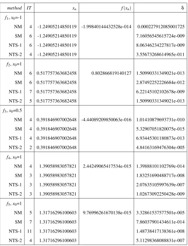
4. Numerical Examples

We present some example to illustrate the root of the newly developed two step iterative method, see Table 1. We compare the Newton method (NM) and Steffensen’s method (SM).

We suggest the following new two step iterative methods, which will denote by NEW TWO STEP, Theorem 2 (NTS 1) and Theorem 4 (NTS 2). All computations are performed using MATLAB. The following examples are used for numerical testing.

f₁(x) =sin(x)−1−x3

f₂(x) =cos(x)−xex

f₃(x) =3x−p

1+sin(x)

f₄(x) =cos(x)−√x+1

f5(x) =x+sin(x)−x3

f₆(x) =ex−1.5−tan−1(x)

f₇(x) =xlog₁₀(x)−1.2

f8(x) =sin(x)−1+x

f₁₀(x) =x2−9

As for the convergence criteria, it was required that the distance of two consecutive approx-imations δ and also displayed is the number of iterations to approximate the zero (IT), the

approximate zerox_nand the value f(x_n).

Table 1: ( Numerical Examples and Comprison)

method IT xn f(xn) δ

f1,x0=-1

NM 4 -1.24905214850119 -1.99840144432528e-014 0.000227912085001725

SM 6 -1.24905214850119 7.16056545615724e-009

NTS-1 6 -1.24905214850119 8.06346234227817e-009

NTS-2 4 -1.24905214850119 3.55673268614965e-011

f2,x0=1

NM 6 0.517757363682458 0.802866819140127 1.50990331349021e-013

SM 6 0.517757363682458 2.87492252226684e-012

NTS-1 7 0.517757363682458 6.22145102102678e-009

NTS-2 5 0.517757363682458 1.50990331349021e-013

f3,x0=0.5

NM 4 0.391846907002648 -4.44089209850063e-016 1.01410879693731e-010

SM 4 0.391846907002648 5.32907051820075e-015

NTS-1 4 0.391846907002648 6.93445301180873e-013

NTS-2 2 0.391846907002648 4.84163169476304e-005

f4,x0=1

NM 4 1.39058983057821 2.44249065417534e-015 1.39888101102769e-014

SM 3 1.39058983057821 1.83251690488717e-008

NTS-1 3 1.39058983057821 2.07635105997639e-007

NTS-2 3 1.39058983057821 1.02673092250428e-009

f5,x0=1

NM 5 1.31716296100603 9.76996261670138e-015 3.32861537577501e-005

SM 7 1.31716296100603 7.86037901434611e-014

NTS-1 11 1.31716296100603 1.48738417138361e-008

method IT xn f(xn) δ

f6,x0=1

NM 5 0.767653266201279 0 2.27928786955545e-012

SM 6 0.767653266201279 1.24644738974666e-012

NTS-1 5 0.767653266201279 1.45067710066726e-008

NTS-2 4 0.767653266201279 1.66533453693773e-015

f7,x0=2

NM 4 2.74064609597369 -3.10862446895044e-015 1.70161289503313e-008

SM 5 2.74064609597369 1.16928688953521e-012

NTS-1 5 2.74064609597369 3.6804337355338e-011

NTS-2 3 2.74064609597369 4.51509829524355e-009

f8,x0=1

NM 4 0.510973429388569 -1.11022302462516e-016 3.78060912575862e-008

SM 5 0.510973429388569 4.42400560629608e-010

NTS-1 6 0.510973429388569 9.30553412104019e-011

NTS-2 3 0.510973429388569 1.52370558392789e-008

f9,x0=2.5

NM 3 2.7983604578389 -7.16049482103465e-005 4.63531457597366e-005

SM 6 2.7983604578389 7.59549133810795e-007

NTS-1 5 2.7983604578389 1.19236434058967e-008

NTS-2 3 2.7983604578389 6.77020575017285e-005

f10,x0=2.5

NM 4 3.0000000000000 0.0000000000000 1.67942641127183e-007

SM 7 3.0000000000000 4.97667596022211e-008

NTS-1 5 3.0000000000000 6.03961325396085e-014

NTS-2 4 3.0000000000000 2.40573058363225e-007

5. Conclusion

Conflict of Interests

The authors declare that there is no conflict of interests.

REFERENCES

[1] A. M. Ostrowaki, Solution of Equations and Systems of Equations, Academic Press, New-York, London,

1966.

[2] Aslam Noor, M.. New Family of iterative methods for nonlinear equations, Appl. Math. Computation, 190 (

2007 ): 553 - 558.

[3] H. Azizul, A. Najmuddin, Comparative Study of a new Iterative Method with that of Newton’s Method for

solving algebraic and Transcedental equations, Int. J. Compu. & Math. Sci., 4 (2015), 32 - 37

[4] Chun, C.,. Iterative Methods improving Newton’s method by the decomposition method, Computers Math.

Appl., 50 (2005): 1559-1568.

[5] D. Kincaid, W. Cheney. Numerical Analysis, second ed., Brooks/Cole, Pacific Grove, CA (1996).

[6] F. Soleymani, Optimized Steffensen-Type Methods with Eighth-Order Convergence and High Efficiency

In-dex, Int. J. Math. Math. Sci., 2012 (2012), Article ID 932420.

[7] Householder, A.S.. The Numerical Treatment of a single Nonlinear Equation, McGraw - Hill, New York. (

1970 ).

[8] Jain M. K., Iyengar S.R.K. and Jain R.K., Numerical Methods For Scientific and Engineering Computation,

New Age International Pvt Ltd Publishers (2009).

[9] Kandasamy P., Thilagavathy K., and Gunavathi K., Numerical Methods, S. chand & Company LTD., (2010).

[10] Noor, M. A. , General variational inequalities, Appl. Math. Letters, 1(1988): 119-121.

[11] Noor, M. A., Some developments in general variational inequalities, Appl. Math. Comput.,152(2004):

199-277.

[12] Noor, K. I. and M. A. Noor, Predicot-Corrector Halley method for nonlinear equations, Appl. Math. Comput.,

188(2007):1587-1591.

[13] Noor, M. A., New classes of iterative methods for nonlinear equations, Appl. Math. Computation. 191(2007),

128-131.

[14] Noor, M. A.. On iterative methods for nonlinear equation using homotopy perturbation technique, Appl.

Math. Inform Sci., 4(2011): 227-235.

[15] Noor, M. A., Noor K.I. and Kshif Aftab, Some New Iterative Methods for Solving Nonlinear Equations,

World Applied Sciences Journal 20(2012): 870-874.

[16] Noor, M. A. and K. I. nor, Iterative schemes for solving nonlinear equations, Appl. Math. Computation,

[17] Q. Zheng, j. Wang, P. Zhao and L. Zhang. A Steffensen-like method and its higher - order variants, Applied

Mathematics and Computation, 214(2009), 10-16.

[18] X. Feng, Y. He, High order iterative methods without derivatives for solving nonlinear equations, Applied