Volume 16, Number 6 (2018), 822-841
URL:https://doi.org/10.28924/2291-8639 DOI:10.28924/2291-8639-16-2018-822
NEW MODIFIED METHOD OF THE CHEBYSHEV COLLOCATION METHOD FOR SOLVING FRACTIONAL DIFFUSION EQUATION
H. JALEB, H. ADIBI∗
Department of Mathematics, Central Tehran Branch, Islamic Azad University, Tehran, Iran
∗Corresponding author: [email protected]
Abstract. In this article a modification of the Chebyshev collocation method is applied to the solution of space fractional differential equations. The fractional derivative is considered in the Caputo sense. The finite difference scheme and Chebyshev collocation method are used. The numerical results obtained by this approach have been compared with other methods. The results show the reliability and efficiency of the proposed method.
1. Introduction
The fractional partial differential equations (FPDEs) arise in numerous problems of engineering, physics,
mathematics, chemistry, biology,and viscoelasticity ( [1], [2], [3], [4]).Most fractional differential equations
do not have exact analytical solutions, thus many authors are seeking ways to numerically solve these
problems( [5], [6]).
Recently, some different methods to solve fractional differential equations have been given such as variational
iteration method [7], homotopy perturbation method [8], adomian decomposition method [9], homotopy
analysis method [10], and collocation method [11]. A least square finite element solution of a fractional-order
two-point boundary value problems, developed in [12]. Sumudu transform method for solving fractional
differential equations and fractional diffusion-wave equation as well proposed in [13]. Wavelet operational
Received 2017-10-18; accepted 2017-12-16; published 2018-11-02. 2010Mathematics Subject Classification. 34A08.
Key words and phrases. fractional diffusion equation; Caputo derivative; fractional Riccati differential equation; finite difference; collocation; Chebyshev polynomials.
c
2018 Authors retain the copyrights of their papers, and all open access articles are distributed under the terms of the Creative Commons Attribution License.
fractional Fokker-Planck equation into a system of ordinary differential equations suggested in( [15], [16]) .The
space fractional diffusion equations are solved numerically .Khader proposed Chebyshev collocation method
to discretize space fractional diffusion equations to obtain a linear system of ordinary differential equations
and he solved the resulting system by finite difference method [17]. Saadatmandi and et al. [18]applied Tau
approach to solve space fractional diffusion equations.
2. Basic ideas and definitions
Definition 2.1. The Caputo fractional derivative operator C0Dxα of order αis defined in the following
form [4]:
C
0Dxαf(x) =
1 Γ(m−α)
Rx
0
f(m)(t)
(x−t)α−m+1dt, α >0,
wherem−1< α≤m, m∈N, x >0.
Caputo fractional derivative operator is a linear operation and for the Caputo derivative we have [19]:
C
0D
α
xc= 0, (2.1)
C
0D
α xx
n=
0, n∈N0 and n <dαe, Γ(n+1)
Γ(n+1−α)x
n−α, n∈N
0 and n≥ dαe,
(2.2)
wherecis a constant anddαedenotes the smallest integer greater than or equal toαandN0={1,2, ...}.For
α∈N0,the Caputo differential operator coincides with the usual differential of integer order ( [19], [20], [21]).
Definition 2.2.Theweighted−LPnorm is defined in the following form [22]:
kukLpw(−1,1)= (
Z 1 −1
|u(x)|pw(x)dx)1/pf or 1≤p <∞, (2.3)
and we again set
kukL∞
w(−1,1)= sup
−1≤x≤1
|u(x)|=kukL∞(−1,1). (2.4)
Definition 2.3.We define natural Sobolev norms as follows [22]:
kukHm
w(−1,1)= (
m X
k=0
ku(k)k2
L2 w(−1,1))
1/2. (2.5)
The Hilbert space associated with this norm is denoted byHm
w(−1,1).we also define the seminorms
|u|Hm,N
w (−1,1)= (
m X
k=min(m,N+1)
ku(k)k2
L2 w(−1,1))
1/2. (2.6)
2.2. A review of the Chebyshev polynomials
The well known Chebyshev polynomials are defined on the interval [-1, 1] as [23]:
T0(z) = 1,
T1(z) =z,
Tn+1(z) = 2zTn(z)−Tn−1(z), n= 1,2, ... .
The analytic form of the Chebyshev polynomialsTn(z) of degree n is given by the following:
Tn(z) =n
[n 2]
X
i=0
(−1)i2n−2i−1(n−i−1)! (i)!(n−2i)!z
n−2i, (2.7)
where [n2] denotes the integer part of n/2. The orthogonality condition is
Z 1 −1
Ti(z)Tj(z)
√
1−z2 dz=
π, f or i=j= 0,
π
2, f or i=j6= 0, 0, f or i6=j.
In order to use these polynomials on the intervalx∈[0,1], we define the so called shifted Chebyshev
poly-nomials by introducing the change of variable z=2x-1.We denoteTn(2x−1) byTn∗(x), defined as:
Tn∗(x) =n n X
k=0
(−1)n−k2
2k(n+k−1)!
(2k)!(n−k)! x
A function u(x), which is squared integrable in [0, 1], may be expressed in terms of shifted Chebyshev
poly-nomials as:
u(x) =
∞ X
i=0
ciTi∗(x),
where
c0= 1
π Z 1
0
u(t)T0∗(x)
√
x−x2 dx, ci= 2
π Z 1
0
u(t)Ti∗(x)
√
x−x2 dx, i= 1,2, ... . (2.9)
Theorem 2.1. [19] Let u(x) be approximated by shifted Chebyshev polynomials as:
um(x) =
m X
i=0
ciTi∗(x), (2.10)
andα >0, then
Dα(um(x)) = m X
i=dαe i X
k=dαe ciw
(α)
i,kx
k−α, (2.11)
wherew(i,kα) is given by:
w(i,kα)= (−1)i−k 2
2ki(i+k−1)!Γ(k+ 1)
(i−k)!(2k)!Γ(k+ 1−α). (2.12)
3. The process of solving the space fractional diffusion equation and modified method
we consider space fractional diffusion equation [17]
∂u(x, t)
∂t =d(x, t)
∂αu(x, t)
∂xα +s(x, t), a < x < b, 0≤t≤M, 1< α≤2, (3.1)
with initial condition
and boundary conditions
u(a, t) =u(b, t) = 0, (3.3)
where the function s(x,t) is a source term.
We use the Chebyshev collocation method to discretize3.1and to get a linear system of ordinary differential
equations and use the finite difference method (FDM) ( [24], [25]) to solve the resulting system, and obtain
the coefficients in the approximate solution. So we approximate u(x,t) as:
um(x, t) = m X
i=0
λi(t)Ti∗(x). (3.4)
From Eqs. 3.1,3.4and using Theorem 2.1 we have:
m X
i=0
dλi(t)
dt T ∗ i(x) =
m X
i=dαe i X
k=dαe
λi(t)wi,k(α)xk−α+s(x, t). (3.5)
Collocating, Eq. 3.5at (m+ 1− dαe) pointsxp yields:
m X
i=0
dλi(t) dt T
∗ i(xp) =
m X
i=dαe i X
k=dαe λi(t)w
(α)
i,kx k−α
p +s(xp, t), P = 0,1, ..., m− dαe. (3.6)
Now we use of roots of shifted Chebyshev PolynomialsTm∗+1−dαe(x) as suitable collocation points.
By substituting Eqs3.4and2.11in the boundary conditions3.3we get
m X
i=0
(−1)iλi(t) = 0, m X
i=0
λi(t) = 0. (3.7)
If so,dαeequations obtained from3.7, along with m+1-dαe equations obtained from3.6 give (m+1)
ordi-nary differential equations which may be solved by using FDM, i=0,1,...,N,τ = MN, 0 ≤ti ≤ M, ti =iτ,
to get the m unknownλi, i=0,1,...,m, in various time levelstn. by determining the unknownsλi(tn) [17],the
approximate m degree polynomials Different time oftn as obtained as follows:
um(x, tn) = m X
i=0
λi(tn)Ti∗(x) =λ n
oT0∗(x) +λ
n
1T1∗(x) +λ
n
2T2∗(x) +...+λ
n mTm∗(x)
in which T is the final time andλni =λi(tn).
To improve the proposed method , Firstly, on average, approximate solution um(x, tn) obtained by
3.8 and the exact solution of problem 3.1,so it new approximate first stage is called and the symbol
uN ewapproximate(1)(x, tn) show. Namely :
uN ewapprox(1)(x, tn) =
1
2[um(x, tn) +uex(x, tn)]. (3.9)
Note thatuex(x, tn)and uapprox(x, tn),respectively are exact solution and approximate solution of the
prob-lem 3.1. At this stage , if |uN ewapprox(1)(x, tn)−uex(x, tn)| to obtain,it is observed that the value of the
amount|uapprox(x, tn)−uex(x, tn) is smaller. In other words, the error between the first stage approximate
and exact solution of the problem, the smaller of ,the error between the approximate solution obtained from
3.8and the exact solution problem.
In the second stage,on average,approximate solution first gain and the exact solution problem and the second
stage is called an New approximation solution, and the symboluN ewapprox(2)(x, tn) show.Namely :
uN ewapprox(2)(x, tn) = 1
2[uN ewapprox(1)(x, tn) +uex(x, tn)]. (3.10)
At this stage , if the value of |uN ewapprox(2)(x, tn)−uex(x, tn| to determine, it will be seen that the value
of the amount |uN ewapprox(1)(x, tn)−uex(x, tn| is smaller. In other words,the error between, the exact
solution and approximate solution of the second stage, is the first step lower. If so, this trend continue, the
average, the approximate solution to the (n-1)th, with the exact solution uex(x, tn) of the problem, it will
be obtained new approximate polynomial and (n)th stage new approximate polynomial is called and the
symboluN ewapprox(n)(x, tn) show , namely:
uN ewapprox(n)(x, tn) =
1
2[uN ewapprox(n−1)(x, tn) +uex(x, tn)]. (3.11)
It will be seen, that the amount of |uN ewapprox(n)(x, tn)−uex(x, tn| is much smaller that the amount
|uapprox(x, tn)−uex(x, tn)|is.So thatuapprox(x, tn) polynomial approximation to the results of the proposed
method is [17].this claim with the numerical results obtained by solving the presented examples shown. In
fact with this work , the numerical solution of equation3.1is improved. The results of numerical examples ,
, for tables, is presented and compared by the several other numerical methods. In this work,the number of
repeat procedures , with the symbol i is shown in the tables.
4. Error analysis and convergence
This section is concerned with the studying of the convergence analysis and getting an upper bound for
the error of the proposed formula.
Theorem 4.1. [19] The error|ET(m)|=|Dαu(x)−Dαum(x)| in approximatingDαu(x) byDαum(x)is
bounded as:
|ET(m)| ≤ | ∞ X
i=m+1
ci(
i X
k=dαe k−dαe
X
j=0
θi,j,k)|, (4.1)
where
θi,j,k= (−1)i
−k2i(i+k−1)!Γ(k−α+1 2)
hjΓ(k+12)(i−k)!Γ(k−α−j+1)Γ(k+j−α+1)
, j= 1,2, ... .
Theorem 4.2. (Chebyshev truncation theorem) .The truncation erroru(x)−uN(x),whereuN(x) =PNk=0ckTk∗(x),
is the truncated Chebyshev series of u, satisfies the inequality [22]:
ku(x)−uN(x)kLpw(−1,1)≤CN
−m
m X
k=min(m,N+1)
ku(k)k
Lpw(−1,1), f or1≤p <∞, (4.2)
for all functions u whose distributional derivatives of order up to m belong toLpw(−1,1). C is a constant and
depends on m.
If so, whenN → ∞,we have:
0≤ lim
N−→∞(ku(x)−uN(x)kL
p
w(−1,1))≤Nlim−→∞(CN
−m
m X
k=min(m,N+1)
ku(k)k
Lpw(−1,1)), (4.3)
In the equation4.3, if max|Pmk=min(m,N+1)ku(k)k
Lpw(−1,1)| ≤M,weher M dimension is fixed, in the case we
have: limN−→∞(CN−mPmk=min(m,N+1)ku (k)k
Lpw(−1,1)) = 0.
Then, according equation4.3, and according to the squeeze theorem, we have:
limN−→∞(ku(x)−uN(x)kLpw(−1,1)) = 0.
Now, to discuss modified method error analysis is presented, polynomial approximations obtained3.8of
the proposed approach [17],P0(x, tn) call. Namely:
P0(x, tn) =um(x, tn) =
m X
i=0
λi(tn)Ti∗(x). (4.4)
so we have:
|P0(x, tn)−uex(x, tn)| ≤ε0, (4.5)
If you put
uN ewapprox(1)(x, tn) = 1
2[um(x, tn) +uex(x, tn)] =P1(tn), (4.6) we have:
|P1(x, tn)−uex(x, tn)| ≤ε1. (4.7)
Considering the ties4.5,4.6and4.7, we have:
|P1(x, tn)−uex(x, tn)| ≤ε1⇒ | 1
2[P0(x, tn) +uex(x, tn)]−uex(x, tn)| ≤ε1
⇒ |P0(x, tn)−uex(x, tn)| ≤2ε1≤ε0,
so the result is:
ε1≤
ε0
2. (4.8)
For these arrangements, ifuN ewapprox(2)(x, tn) = 12[um(x, tn) +uex(x, tn)] toP2(tn) call, you can write:
|P2(x, tn)−uex(x, tn)| ≤ε2⇒ | 1
⇒ |P1(x, tn)−uex(x, tn)| ≤2ε2⇒ | 1
2[P0(x, tn) +uex(x, tn)]−uex(x, tn)| ≤2ε2
⇒ |P0(x, tn)−uex(x, tn)| ≤2×2ε2≤ε0,
so the result is:
ε2≤
ε0
22. (4.9)
By following this process, the n-th stage will be:
εn≤ ε0
2n. (4.10)
In fact, ifPn(x, tn) polynomial approximation is made in step n, we get the following result:
|Pn(x, tn)−uex(x, tn)| ≤εn≤ ε0
2n. (4.11)
For4.11, can be written:
0≤ lim
n→∞(|Pn(x, tn)−uex(x, tn)|)≤nlim→∞( ε0
2n), (4.12)
then, according equation4.12, and according to the squeeze theorem, we have:
lim
n→∞(|Pn(x, tn)−uex(x, tn|) = 0.
ferential equation.also
Dαu(t) +u2(t)−1 = 0, t >0,0< α≤1,
with the initial conditionu(0) =u0,
in next section we illustrated this approach by example 5.1.
5. Numerical results
Example 5.1. Consider the fractional Riccati differential equation of the form
Dαu(t) +u2(t)−1 = 0, t >0, 0< α≤1, (5.1)
with the initial condition
u(0) =u0, (5.2)
and the parameterα, refers to the fractional order of the time derivative.
Forα= 1; the Eq.5.1is the standard Riccati differential equation
du(t)
dt +u
2(t)−1 = 0.
The exact solution to this equation is
u(t) = e 2t−1 e2t+ 1.
Now we approximate the function u(t) by using formula??and its Caputo derivativeDαu(t) by using the
presented formula2.11with m=5.Then fractional Riccati differential equation5.1is transformed to the
fol-lowing approximated form:
5
X
i=1
i X
k=1
ciwi,k(α)tk−α+ ( 5
X
i=0
wherewi,k(α)is defined in2.12.
Also the initial condition5.2is given by :
5
X
i=0
ci(Ti∗(0)) =u0. (5.4)
We now collocate Eq.5.3at (m+ 1− dαe) pointstp as:
5
X
i=1
i X
k=1
ciw(i,kα)tkp−α+ (
5
X
i=0
ciTi∗(tp))
2
−1 = 0, p= 0,1,2,3,4. (5.5)
Note thatt,
psare roots of shifted Chebyshev polynomialT5∗(t), i.e.
t0= 0.5, t1= 0.206107, t2= 0.793893, t3= 0.024471, t4= 0.975528.
By using Eqs.5.4and 5.5, we obtain a system of non-linear algebraic equations which contains 6 equations
for the unknownsci, i= 0,1, ...,5.
By solving the previous system, utilizing the Newton iteration method, we obtain the unknown ci, i =
0,1, ...,5,and therefore, the approximate solution is obtained via:
u5(t) = 5
X
i=0
ciTi∗(t). (5.6)
Forα= 1 , and then determine the coefficientsci about5.6, polynomial approximation as follows:
u5(t) = 5
X
i=0
ciTi∗(t) = 2.66714×10⁻¹⁷+ 0.999372x+ 0.0157609x2−0.41893x3+ 0.180634x4−0.0152477x5.
(5.7)
In this way, the improved method described for polynomial approximation5.7was used. In the table 1, 2 the
numerical results and absolute error between the exact solutionuex, and the approximate solutionuapprox
modified method
x i=0 i=10 i=20 i=30 i=35
|Error(0)| |Error(10)| |Error(20)| |Error(30)| |Error(35)|
0.0 2.66714×10⁻¹⁷ 0.00000 0.00000 0.00000
0.1 2.58369×10⁻⁵ 2.52314×10⁻⁸ 2.46400×10⁻¹¹ 2.39808×10⁻¹⁴ 6.93889×10⁻¹⁶
0.2 6.22951×10⁻⁵ 6.08351×10⁻⁸ 5.94093×10⁻¹¹ 5.80924×10⁻¹⁴ 1.77636×10⁻¹⁶
0.3 3.25723×10⁻⁵ 3.18089×10⁻⁸ 3.10634×10⁻¹¹ 3.02536×10⁻¹⁴ 9.43690×10⁻¹⁶
0.4 2.16611×10⁻⁵ 2.11534×10⁻⁸ 2.06575×10⁻¹¹ 2.02061×10⁻¹⁴ 6.10623×10⁻¹⁶
0.5 4.38002×10⁻⁵ 4.27737×10⁻⁸ 4.17711×10⁻¹¹ 4.06897×10⁻¹⁴ 1.27676×10⁻¹⁵
0.6 1.64887×10⁻⁵ 1.61022×10⁻⁸ 1.57249×10⁻¹¹ 1.53211×10⁻¹⁴ 4.44089×10⁻¹⁶
0.7 3.04507×10⁻⁵ 2.97370×10⁻⁸ 2.90398×10⁻¹¹ 2.84217×10⁻¹⁴ 6.66134×10⁻¹⁶
0.8 4.75369×10⁻⁵ 4.64228×10⁻⁸ 4.53346×10⁻¹¹ 4.44089×10⁻¹⁴ 1.33227×10⁻¹⁵
0.9 1.43902×10⁻⁵ 1.40529×10⁻⁸ 1.37235×10⁻¹¹ 1.35447×10⁻¹⁴ 4.44089×10⁻¹⁶
1.0 3.98000×10⁻⁶ 3.88672×10⁻⁸ 3.79574×10⁻¹² 3.77476×10⁻¹⁵ 2.22045×10⁻¹⁶
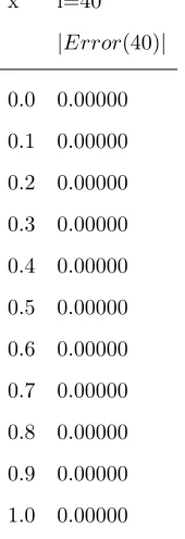
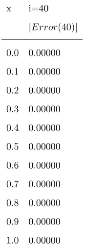
Table 2: comparison of absolute errors for u(x)at m=5 with different values of i for example 5.1. by
modified method
x i=40
|Error(40)|
0.0 0.00000
0.1 0.00000
0.2 0.00000
0.3 0.00000
0.4 0.00000
0.5 0.00000
0.6 0.00000
0.7 0.00000
0.8 0.00000
0.9 0.00000
Example 5.2. In this section, we consider space fractional diffusion equation3.1withα= 1.8, of the form:
∂u(x, t)
∂t =d(x, t)
∂1.8u(x, t)
∂x1.8 +s(x, t),
where, 0< x <1, with the diffusion coefficient: d(x,t)= Γ(1.2)x1.8, and the source function: s(x,t)=3x2(2x−
1)e−t. The initial and boundary conditions are respectively as:
u(x,0)=x2(1−x),
u(0,t)=u(1,t)=0.
The exact solution of this problem is u(x,t)=x2(1−x)e−t.
We apply the present method with m=3, and approximate the solution as follows:
u3(x, t) = 3
X
i=0
λi(t)Ti∗(x). (5.8)
In5.8, after determining the coefficientsλi(t) for T=2 [17], Polynomial approximation is as follows.
u3(x,2) = 3
X
i=0
λi(t800)Ti∗(x) = ´λ800o + ´λ8001 x+ ´λ8002 x2+ ´λ8003 x3=
−8.673617−19+ 0.000894x+ 0.134649x2−0.135543x3 (5.9)
In Table3, the absolute error, between the exact solutionuex and the approximate solutionuapprox at m=3
and time stepτ = 0.0025,with the final time T=2 is given. Also, In the table 4, 5 ,6 the numerical results
and absolute error between the exact solutionuex, and the approximate solutionuapproxwith different values
of i, by means of the proposed modified method are given.
It is notable that by consideringτ= 0.0025,and using finite differential method (FDM) about5.8[17], we
will has 800 (Tτ = 0.00252 = 800) level time for approximate solutionsu(x, tn), 0< x <1.
In the above example all 800 values ofu(x, tn) are calculated by utilizing mathematica.
Example 5.3. [16]In this example, we consider the following space fractional diffusion equation
∂u(x, t)
∂t =P(x)
∂αu(x, t)
∂xα +s(x, t), 0< x <1 (5.10)
with initial conditionu(x,0) =x4,
x Modified method Method[17] Method [26] Method [18]
0.0 2.46519×10⁻³² 1.70849×10⁻⁴ 4.483787×10⁻³ 0.00
0.1 2.60209×10⁻¹⁸ 2.10940×10⁻⁵ 4.479660×10⁻³ 2.89×10⁻⁵
0.2 5.20417×10⁻¹⁸ 1.76609×10⁻⁴ 4.201329×10⁻³ 1.09×10⁻⁴
0.3 8.67362×10⁻¹⁸ 3.01420×10⁻⁴ 3.695172×10⁻³ 2.20×10⁻⁴
0.4 1.04083×10⁻¹⁷ 4.04138×10⁻⁴ 3.007566×10⁻³ 3.40×10⁻⁴
0.5 1.38778×10⁻¹⁷ 4.89044×10⁻⁴ 2.184889 ×10⁻³ 4.45×10⁻⁴
0.6 2.08167×10⁻¹⁷ 4.89044×10⁻⁴ 1.273510 ×10⁻³ 5.15×10⁻⁴
0.7 1.38778×10⁻¹⁷ 5.63305×10⁻⁴ 0.319831 ×10⁻³ 5.27×10⁻⁴
0.8 1.38778×10⁻¹⁷ 6.33367×10⁻⁴ 0.629793 ×10⁻³ 4.60×10⁻⁴
0.9 2.77556×10⁻¹⁷ 7.05677×10⁻⁴ 1.528978 ×10⁻³ 2.91×10⁻⁴
1.0 0.00000 8.82821×10⁻⁴ 2.331347 ×10⁻³ 0.00
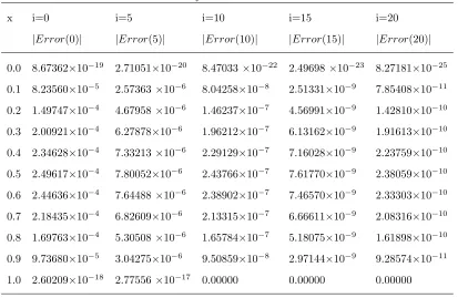
Table 4: Comparison of absolute errors for u(x,2)at m=3 and T=2 with different values of i for example
5.2. by modified method
x i=0 i=5 i=10 i=15 i=20
|Error(0)| |Error(5)| |Error(10)| |Error(15)| |Error(20)|
0.0 8.67362×10⁻¹⁹ 2.71051×10⁻²⁰ 8.47033×10⁻²² 2.49698×10⁻²³ 8.27181×10⁻²⁵
0.1 8.23560×10⁻⁵ 2.57363×10⁻⁶ 8.04258×10⁻⁸ 2.51331×10⁻⁹ 7.85408×10⁻¹¹
0.2 1.49747×10⁻⁴ 4.67958×10⁻⁶ 1.46237×10⁻⁷ 4.56991×10⁻⁹ 1.42810×10⁻¹⁰
0.3 2.00921×10⁻⁴ 6.27878×10⁻⁶ 1.96212×10⁻⁷ 6.13162×10⁻⁹ 1.91613×10⁻¹⁰
0.4 2.34628×10⁻⁴ 7.33213×10⁻⁶ 2.29129×10⁻⁷ 7.16028×10⁻⁹ 2.23759×10⁻¹⁰
0.5 2.49617×10⁻⁴ 7.80052×10⁻⁶ 2.43766×10⁻⁷ 7.61770×10⁻⁹ 2.38059×10⁻¹⁰
0.6 2.44636×10⁻⁴ 7.64488×10⁻⁶ 2.38902×10⁻⁷ 7.46570×10⁻⁹ 2.33303×10⁻¹⁰
0.7 2.18435×10⁻⁴ 6.82609×10⁻⁶ 2.13315×10⁻⁷ 6.66611×10⁻⁹ 2.08316×10⁻¹⁰
0.8 1.69763×10⁻⁴ 5.30508×10⁻⁶ 1.65784×10⁻⁷ 5.18075×10⁻⁹ 1.61898×10⁻¹⁰
0.9 9.73680×10⁻⁵ 3.04275×10⁻⁶ 9.50859×10⁻⁸ 2.97144×10⁻⁹ 9.28574×10⁻¹¹
1.0 2.60209×10⁻¹⁸ 2.77556×10⁻¹⁷ 0.00000 0.00000 0.00000
u(0, t) = 0, u(1, t) =e−t,
where the functions(x, t) =−2e−tx4is a source term, andP(x) =241Γ(5−α).
The exact solution to this equation ise−tx4.
Table 5: Comparison of absolute errors for u(x,2)at m=3 and T=2 with different values of i for example
5.2. by modified method
x i=25 i=30 i=35 i=40 i=45
|Error(25)| |Error(30)| |Error(35)| |Error(40)| |Error(45)|
0.0 2.58494×10⁻²⁶ 8.07794×10⁻²⁸ 2.52435×10⁻²⁹ 7.88861×10⁻³¹ 2.46519×10⁻³²
0.1 2.45440×10⁻¹² 7.66997×10⁻¹⁴ 2.39674×10⁻¹⁵ 7.45931×10⁻¹⁷ 2.60209×10⁻¹⁸
0.2 4.46280×10⁻¹² 1.39462×10⁻¹³ 4.35763×10⁻¹⁵ 1.35308×10⁻¹⁶ 5.20417×10⁻¹⁸
0.3 5.98792×10⁻¹² 1.87123×10⁻¹³ 5.84775×10⁻¹⁵ 1.82146×10⁻¹⁶ 8.67362×10⁻¹⁸
0.4 6.99246×10⁻¹² 2.18513×10⁻¹³ 6.82440×10⁻¹⁵ 2.11636×10⁻¹⁶ 1.04083×10⁻¹⁷
0.5 7.43915×10⁻¹² 2.32474×10⁻¹³ 7.25808×10⁻¹⁵ 2.22045×10⁻¹⁶ 1.38778×10⁻¹⁷
0.6 7.29072×10⁻¹² 2.27839×10⁻¹³ 7.11237×10⁻¹⁵ 2.22045×10⁻¹⁶ 2.08167×10⁻¹⁷
0.7 6.50988×10⁻¹² 2.03434×10⁻¹³ 6.35603×10⁻¹⁵ 1.94289×10⁻¹⁶ 1.38778×10⁻¹⁷
0.8 5.05931×10⁻¹² 1.58096×10⁻¹³ 4.92661×10⁻¹⁵ 1.52656×10⁻¹⁶ 1.38778×10⁻¹⁷
0.9 2.90179×10⁻¹² 9.06775×10⁻¹⁴ 2.83107×10⁻¹⁵ 6.93889×10⁻¹⁷ 2.77556×10⁻¹⁷
1.0 0.00000 0.00000 0.00000 0.00000 0.00000
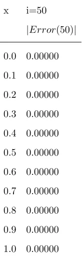
Table 6: comparison of absolute errors for u(x,2)at m=3 and T=2 with different values of i for example 5.2.
by modified method
x i=50
|Error(50)|
0.0 0.00000
0.1 0.00000
0.2 0.00000
0.3 0.00000
0.4 0.00000
0.5 0.00000
0.6 0.00000
0.7 0.00000
0.8 0.00000
0.9 0.00000
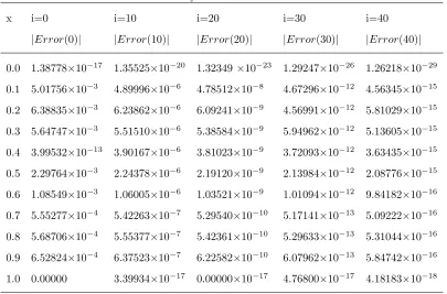
5.2. by modified method
x i=0 i=10 i=20 i=30 i=40
|Error(0)| |Error(10)| |Error(20)| |Error(30)| |Error(40)|
0.0 1.38778×10⁻¹⁷ 1.35525×10⁻²⁰ 1.32349×10⁻²³ 1.29247×10⁻²⁶ 1.26218×10⁻²⁹
0.1 5.01756×10⁻³ 4.89996×10⁻⁶ 4.78512×10⁻⁸ 4.67296×10⁻¹² 4.56345×10⁻¹⁵
0.2 6.38835×10⁻³ 6.23862×10⁻⁶ 6.09241×10⁻⁹ 4.56991×10⁻¹² 5.81029×10⁻¹⁵
0.3 5.64747×10⁻³ 5.51510×10⁻⁶ 5.38584×10⁻⁹ 5.94962×10⁻¹² 5.13605×10⁻¹⁵
0.4 3.99532×10⁻¹³ 3.90167×10⁻⁶ 3.81023×10⁻⁹ 3.72093×10⁻¹² 3.63435×10⁻¹⁵
0.5 2.29764×10⁻³ 2.24378×10⁻⁶ 2.19120×10⁻⁹ 2.13984×10⁻¹² 2.08776×10⁻¹⁵
0.6 1.08549×10⁻³ 1.06005×10⁻⁶ 1.03521×10⁻⁹ 1.01094×10⁻¹² 9.84182×10⁻¹⁶
0.7 5.55277×10⁻⁴ 5.42263×10⁻⁷ 5.29540×10⁻¹⁰ 5.17141×10⁻¹³ 5.09222×10⁻¹⁶
0.8 5.68706×10⁻⁴ 5.55377×10⁻⁷ 5.42361×10⁻¹⁰ 5.29633×10⁻¹³ 5.31044×10⁻¹⁶
0.9 6.52824×10⁻⁴ 6.37523×10⁻⁷ 6.22582×10⁻¹⁰ 6.07962×10⁻¹³ 5.84742×10⁻¹⁶
1.0 0.00000 3.39934×10⁻¹⁷ 0.00000×10⁻¹⁷ 4.76800×10⁻¹⁷ 4.18183×10⁻¹⁸
u4(x,1) = 4
X
i=0
λi(t)Ti∗(x) = 1.38778×10−
17+ 0.074363x
−0.274432x2+ 0.339516x3+ 0.228432x4, (5.11)
note that, in this example ∆t= 0.001 is considered.
Now apply improved method for polynomial approximation expression5.11,absolute error between the exact
solution, and new approximate solution obtained based on the number of repetitions of the process, shown
in Tables 7 and 8.
Example 5.4. [15]consider the following space fractional diffusion equation
∂u(x, t)
∂t =P(x)
∂1.5u(x, t)
∂x1.5 +s(x, t), 0< x <1 (5.12)
with the initial condition
u(x,0) = (x2+ 1) sin(1),
and boundary conditions
u(0, t) sin(t+ 1), u(1, t) = 2 sin(t+ 1), f or t >0,
Table 8: Comparison of absolute errors for u(x,1)at m=4 and T=1 with different values of i for example
5.2. by modified method
x i=50 i=60 i=70 i=80
|Error(50)| |Error(60)| |Error(70)| |Error(80)|
0.0 1.23260×10⁻³² 1.20371×10⁻³⁵ 1.17549×10−38 1.14794×10−41
0.1 4.46548×10⁻¹⁸ 4.06965×10⁻²¹ 3.97427×10⁻²⁴ 3.88112×10⁻²⁷
0.2 5.73658×10⁻¹⁸ 3.37867×10⁻²¹ 3.29948×10⁻²⁴ 3.222151×10⁻²⁷
0.3 5.24988×10⁻¹⁸ 2.07294×10⁻²¹ 2.02436×10⁻²⁴ 1.97691×10⁻²⁷
0.4 4.76720×10⁻¹⁸ 1.22852×10⁻²⁰ 1.19973×10⁻²³ 1.17161×10⁻²⁶
0.5 3.31277×10⁻¹⁸ 2.72581×10⁻²⁰ 2.66192×10⁻²³ 2.59953×10⁻²⁶
0.6 4.52895×10⁻¹⁹ 4.69916×10⁻²⁰ 4.58902×10⁻²³ 4.48146×10⁻²⁶
0.7 3.81242×10⁻¹⁸ 7.14857×10⁻²⁰ 6.98103×10⁻²³ 6.81741×10⁻²⁶
0.8 3.56196×10⁻¹⁷ 1.00740×10⁻¹⁹ 9.83794×10⁻²³ 9.60736×10⁻²⁶
0.9 2.85435×10⁻¹⁷ 1.34756×10⁻¹⁹ 1.31598×10⁻²² 1.28513×10⁻²⁵
1.0 1.11632×10⁻¹⁷ 1.73532×10⁻¹⁹ 1.69465×10⁻²² 1.65493×10⁻²⁵
andP(x) = Γ(1.5)x0.5.
The exact solution of this problem isu(x, t) = (x2+ 1) sin(t+ 1).
By applying the proposed method [17] , polynomial approximation is as follows:
u2(x,1) = 2
X
i=0
λi(t)Ti∗(x) = 0.909297 + 0.00049296x+ 0.908804x2, (5.13)
note that, in this example ∆t= 0.001 is considered.
Now apply improved method for polynomial approximation expression 5.13. Absolute error between the
exact solution, and new approximate solution obtained based on the number of repetitions of the process,
shown in Tables 9 and 10.
6. Conclusion
In this paper, we proposed a new modified of numerical method ,based on the shifted Chebyshev collocation
method and finite difference scheme, to find the solution of the space fractional diffusion equations and
fractional Riccati differential equation. In this method, the fractional derivatives are described in the Caputo
sense. Comparison between our proposed method and other methods , shows that this scheme is superior
5.4. by modified method
x i=0 i=10 i=20 i=30 i=38
|Error(0)| |Error(10)| |Error(20)| |Error(30)| |Error(38)|
0.0 2.22×10⁻¹⁸ 0.00000 0.00000 0.00000 0.00000
0.1 4.43×10⁻⁵ 4.33266×10⁻⁸ 4.23110×10⁻¹¹ 4.13003×10⁻¹⁴ 2.22054×10⁻¹⁶
0.2 7.89×10⁻⁵ 7.70250×10⁻⁸ 7.52197×10⁻¹¹ 7.33857×10⁻¹⁴ 2.22045×10⁻¹⁶
0.3 1.03×10⁻⁴ 1.01095×10⁻⁷ 9.87258×10⁻¹¹ 9.63674×10⁻¹⁴ 3.33067×10⁻¹⁶
0.4 1.18×10⁻⁴ 1.15538×10⁻⁷ 1.12830×10⁻¹¹ 1.10134×10⁻¹³ 3.33067×10⁻¹⁶
0.5 1.23×10⁻⁴ 1.20352×10⁻⁷ 1.17531×10⁻¹¹ 1.14797×10⁻¹³ 4.44089×10⁻¹⁶
0.6 1.18×10⁻⁴ 1.15538×10⁻⁷ 1.12830×10⁻¹¹ 1.10245×10⁻¹³ 6.66134×10⁻¹⁶
0.7 7.89×10⁻⁴ 1.01095×10⁻⁷ 9.87258×10⁻¹¹ 9.62563×10⁻¹⁴ 2.22045×10⁻¹⁶
0.8 4.43×10⁻⁴ 7.70250×10⁻⁷ 7.52197×10⁻¹¹ 7.32747×10⁻¹⁴ 2.22045×10⁻¹⁶
0.9 4.43×10⁻¹⁶ 4.33266×10⁻⁸ 4.23110×10⁻¹¹ 4.13003×10⁻¹⁴ 2.22045×10⁻¹⁶
1.0 2.22×10⁻¹⁶ 0.00000 0.00000 0.00000 0.00000
Table10: Comparison of absolute errors for u(x,1)at m=2 and T=1 with different values of i for example
5.4. by modified method
x i=40
|Error(40)|
0.0 0.00000
0.1 0.00000
0.2 0.00000
0.3 0.00000
0.4 0.00000
0.5 0.00000
0.6 0.00000
0.7 0.00000
0.8 0.00000
0.9 0.00000
7. Acknowledgements
It should be mentioned that the above article has been derived from Ph.D thesis, at the Islamic Azad
University Central Tehran Branch.
References
[1] L. Bagley and P. J. Torvik, On the appearance of the fractional derivative in the behavior of real materials, J. Appl. Mech, 51(19840), 294-298.
[2] K. B. Oldham and J. Spanier, The Fractional Cvalculus, Academic Press, New York and London, ( 1974).
[3] K. S. Miller and B. Ross, An Introduction to the Fractional Calculus and Fractional Differential Equations, John Wiley, New York, (1993).
[4] S. G. Samko, A.A. Kilbas and O.I. Marichev, Fractional Integrals and Derivatives: Theory and Applications, Gordon and Breach Science Publishers, USA, (1993).
[5] S. Das, Fractional Calculus for System Identification and Controls, Springer, New york, (2008).
[6] H. Sweilam and M. M. Khader, A Chebyshev pseudo-spectral method for solving fractional integro-differential equations, ANZIAM J.51(2010), 464-475.
[7] M. Inc, The approximate and exact solutions of the space-and time-fractionalBurger,sequations with initial conditions
by varational iteration method, J. Math. Anal. Appl.345(2008), 476-484.
[8] N. H. Sweilam, M.M.Khader and R.F. AL-Bar, Numerical studies for a multi-order fractional differential equation, Phys. Lett. A,371(2007), 26-33.
[9] H. Jafari and V. Daftardar-Gejji, Solving linear and nonlinear fractional diffusion and wave equations by ADM, Appl. Math. Comput,180(2006), 488-497.
[10] I. Hashim, O. Abdulaziz and S. Momani, Homotopy analysis method for fractional IVPs, Commun. Nonlinear Sci. Numer. Simul.14(2009), 674-684.
[11] E. A. Rawashdeh, Numerical solution of fractional integro-differential equations by collocation method, Appl. Math. Com-put,176(2006), 1-6.
[12] G. J. Fix, J.P. Roop,Least squares finite element solution of the fractional order two-point boundary value problem, Com-put. Math. Appl.48(2004), 1017-1033.
[13] R. Darzi, B.Mohammadzade, S.Musavi, R.Behshti, Sumudu transform method for solving fractional differential equations and fractional diffusion-Wave equation, J. Math. Comput. Sci.6(2013) 79-84.
[14] A. Neamaty, B. Agheli, R. Darzi, Solving fractional partial differential equation by using wavelet operational method, J. Math. Comput. Sci.7(2013), 230-240 .
[15] F. Liu, V .Anh and I. Turner,Numerical solution of the space fractional Fokker-Plank equation, J. Comput. Appl. Math. 166(2004), 209-219.
[16] F. Liu, V. Anh, I. Turner, P. Zhuang, Time fractional advection dispersion equation, J. Appl. Math. Comput.13(2003), 233-245.
Appl.62(2011), 1135-1142.
[19] M. M. Khader, N. H. Swetlam and A. M. S. Mahdy, The Chebyshev collection method for solving fractional order Klein-Gordon equation, Wseas Trans. Math.13(2014), 2224-2880 .
[20] I. Podlubny, Fractional Differential Equations, Academic Press, New York, (1999).
[21] M. Joseph Kimeu, Fractional Calculus: Definitions and Applications, Western Kentucky University, (2009).
[22] C. Canuto, A. Quarteroni, M. Y. Hussaini, and T. A. Zang, Spectral Methods Fundamentals in Single Domains, Springer-Verlag Berlin Heidelberg, Printed in Germany (2006).
[23] M. A.Snyder, Chebyshev Methods in Numerical Approximation, Prentice-Hall, Inc. Englewood Cliffs, N. J. (1966). [24] M. M. Meerschaert and C. Tadjeran,Finite difference approximations for fractional advection-dispersion flow equations, J.
Comput. Appl. Math.172(2008), 65-77.
[25] M. M. Meerschaert and C. Tadjeran, Finite difference approximations for two-sided space-fractional partial differential equations, Appl. Numer. Math.56(2006), 80-90.