Comparing the ANN and Linear Regression in
Estimation of the Growth Model (The Case of MENA)
Majid Sameti∗ Shekoofeh Farahmand∗∗
Keihan Koleyni∗∗∗ Roya Aghaeifar∗∗∗∗
Received: 2011/06/25 Accepted: 2012/04/23
Abstract
conomic convergence is one of the important topics of new macroeconomics. It refers to tendency of income per capita of countries (regions) to converge to their steady-state value. There are two kinds of convergence: conditional and absolute convergence. This paper examines income convergence between 22 MENA countries during the period of 1970-2003 by using the neoclassical growth model of Barro-Salla-i-Martin for both kinds of convergence. Non-linearity of the underlying relationships, the restrictiveness of assumptions of functional forms and econometric problems in the estimation and application of theoretical models advocate for the use of Artificial Neural Networks (ANN) algorithms. We show that by changing the quantitative tools of analysis and using ANN, the results become more precise. Results show that absolute convergence and conditional convergence are significant but the rate of convergence is low.
Keywords: Income Convergence, MENA Countries, Artificial Neural Networks
1- Introduction
Movement of the world toward integration, polarization and regional formation of blocks are current problems. Debates about integrations such as European, Islamic, G7 or ASEAN countries can be studied in different fields
∗ Associate Professor, University of Isfahan, (Corresponding Author).
∗∗ Assistant Professor, University of Isfahan. ∗∗∗ Ph.D. student, University of Memphis. ∗∗∗∗ M.A. of Economics.
of economic emphasis. Income (output) convergence is one of the interesting problems of new macroeconomics. It refers to tendency of per capita income of countries (regions) to converge to their steady- state value.
Convergence hypothesis tries to answer two main questions. First, do the poor countries (regions) grow faster than rich ones? That depends on the effect of initial conditions on per capita income differences across countries and the speed of convergence, which introduced by β -convergence in growth literature. Second, one can ask whether the dispersion of per capita income of countries (regions) is decreasing over the time or not. This type of convergence, called σ-convergence, focuses less on initial conditions, and instead emphasizes income distribution by measuring standard deviations. For studying β-convergence, two kinds of convergence should be studied: conditional and absolute convergence. If the differences in per capita income are temporary, and solely because of initial conditions absolute convergence is occurring. If the differences are permanent because of cross-country structural heterogeneity, the conditional convergence is occurring (Durlauf et al., 2005). Expansion of literature on economic growth, its modeling, and the development of additional quantitative tools of analysis and different type of statistical information that can be used for quantitative analysis (cross-section, time series or panel data) have promoted a large body of empirical studies about convergence hypothesis. However, still some critics about both kinds of β
We try to solve these questions about non-linearity of the underlying relationships and ambiguity of functional form by using non-parametric approach of Artificial Neural Networks (ANN). We show that by changing the quantitative tools of analysis from traditional econometric tools to Artificial Neural Networks (ANN), the results will become more precise and the non-linearity problem will be solved and appropriate functional form of movements of per capita income of countries toward their steady-state value will be gained. We used Multilayered Feed-forward Networks for this purpose and compared it with OLS estimation method based on cross-country regression equations of Barro and Salla-i-Martin model (1990, 1992, and 2004) for both kinds of absolute and conditional
β-convergence during the period of 1970-2003. This paper is organized as follows: in section 2 we discuss some main studies on convergence hypothesis, section 3 declares the methodology and ANN modeling. In section 4, we describe our findings and compare them with OLS method. Finally, section 5 is conclusions.
2-
Literature ReviewAs mentioned before, a large number of studies according to type of data used, the countries in the question, the sample period in the question and choice of control variables exists but we describe here only little part of this huge body of empirics. So many of these empirical studies are based on neoclassical growth models such as Solow (1956), Swan (1956), Koopmans (1956), Cass (1965) and even the older work of Ramsey(1928). In addition, we can see some of studies with endogenous growth models like Jones and Manuelli (1990) and Kelly (1992) but most of endogenous growth models are not compatible with convergence hypothesis like Romer (1986) and Lucas (1988) because of convexity in production function.
i i i i N y In b a N y In N y
In +
ε
⎥ ⎥ ⎦ ⎤ ⎢ ⎢ ⎣ ⎡ + = ⎟ ⎠ ⎞ ⎜ ⎝ ⎛ − ⎟ ⎠ ⎞ ⎜ ⎝ ⎛ 1870 , 1870 , 1979
, (1)
Where, y is the income per capita of countries, N denotes the number of countries, and is the error term.
Barro and Sala-i-Martin (1992) defined β and σ-convergence for US states according to the Solow model. They used the following cross-country regression: it t i it t i
it a e y u
y
y = − − +
⎟ ⎟ ⎠ ⎞ ⎜ ⎜ ⎝ ⎛ − − − ) ( log ). 1 (
log , 1
1 ,
β (2)
Where, the subscript t denotes the year, and the subscript i denotes the country or region, y is income per capita, and u is the error term. If we assume that coefficient is the same for all economies, then . This specification means that the steady state value and the rate of exogenous technological progress are the same for all economies. This assumption is more reasonable for regional data sets than across the world. It is plausible that different regions within a country are more similar than different countries across the world with respect to technology and preferences. Then, as most of researches show, global absolute convergence does not exist. If the intercept is the same for all regions and β > 0, then equation (2) implies that poor economies tend to grow faster than rich ones. This type of convergence is called “absolute” or “unconditional” convergence. If one uses the term (1 ).log(ˆ*)
i y e−β
− as an explanatory
variable it means that the growth rate of economy i depends on its initial level of income and also, depends on the steady state value of income, ˆ*
it i t
i it
t i
it a e y y u
y
y = − − + +
⎟ ⎟ ⎠ ⎞ ⎜ ⎜ ⎝ ⎛
− −
−
) ˆ log( ) log( ). 1 (
log *
1 , 1
,
β (3)
Mankiw, Romer and Weil (1992) used augmented Solow model, which includes accumulation of human as well as physical capital for several large group of countries and found almost the same results as Barro and Sala-i-Martin (1992). Based on Barro and Sala-i-Martin (1992) and cross-section approach, we then see a large body of research. There are also other approaches like time series and panel data analysis. Bernard and Durlauf (1995, 1996), Durlauf (1998), series of Quah’s papers (1993a, 1993b, 1996a, 1996b, 1996c, 1997, and 2001), Nahar and Inder (2002) used time series approach. This approach is largely statistical in nature, and disadvantage of this approach is that it is not according to particular modeled after growth theories.
Lee, Pesaran and Smith (1997), Islam (1995), Caselli, Esquivel and Lefrot (1996), Benhabib and Spiegel (1997), Nerlove (1996), Canova and Marcet (1995), Evans (1998) used panel data approach.The panel data analysis adapts the use of convergence equations as in cross-section analysis. Although, it can help to increase the flexibility of model, the structural error can be seen in this approach.
Efficiency of neural networks is extremely related to architecture and designing of these networks. Different networks with different architecture should be designed and among them, the best network with minimum error should be chosen. In addition, length of studied periods for neural networks is another discussing problem. Usually, neural networks with longer periods are more accurate.
3- Methodology
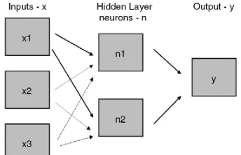
Artificial neural networks are the members of a family of statistical techniques, which try to simulate and model human brain. They have recently received a great deal of attention in many fields of study. A neural network relates a set of input variables (input layers) to a set of one or more output variables (output layers). The component of each layer is called neuron or node.
The difference between a neural network and other approximation methods is that the neural network makes use of one or more hidden layers, in which the input variables are transformed by a special function in parallel processing (McNelis, 2005). Each neuron has one ascendant activation function, which can be linear or nonlinear according to their application. This activation function determine threshold of the neuron.
Figure 1: Architecture of Feed-Forward Networks
This figure shows the architecture of feed-forward back propagation networks. Inputs X makes the first layer of the networks. After this layer, hidden layer with n neurons processes the inputs in parallel. Final layer of a network is output layer.
t i i k i i k t k
x
n
,=
ω
,0+
Σ
*=1ω
, , (4)t ni t k t k
e
n
L
N
, , ,1
1
)
(
−+
=
=
(5)∑
=+
=
* 1 , 0 k k t k k tN
y
γ
γ
(6)
Where,
L
(
n
k,t)
represents the log sigmoid activation function withthe form t i n
e
,1
1
−+
. In addition, the alternative activation function, whichis known as tansig or tanh with the form,
t k t k t k t k n n n n
e
e
e
e
, , , , − −+
−
could be used. In
this system, there are
i
* input variables {x}, andk
* neurons. A linear combination of these input variables observed at time t,{ }
x
i,t,
i
=
1
,...,
i
*,with the coefficient vector or set of input weights
ω
k,i,i
=
1
,...,
i
* , as wellas the constant term
ω
k,0, form the variablen
k,t. This variable istransformed by the activation function, and becomes a neuron
N
k,tattime or observation t. The set of
k
* neurons at time or observation index tare combined in a linear way with the coefficient vector
{ }
y
k,
=
1
,...,
k
*andtaken with constant term
y
0, to form the forecasty
ˆ
t at time t.Figure 2: Architecture of Elman Recurrent Network
This figure shows the architecture of Elman Recurrent networks. Inputs X makes the first layer of the networks. After this layer, hidden layer with n neurons processes the inputs in parallel. Final layer of a network is output layer. This network has a feedback from the hidden layer that works like a memory for network and make the network dynamic.
This network allows the neurons to depend not only on the input variables x, but also on their own lagged values. Thus, the Elman network builds “memory” in the evolution of neurons.The following system represents the recurrent Elman network illustrated in figure 2:
∑
= +∑
= −+
= ,0 *1 , , *1 , 1
,
i i
k
k k kt
t i i k k
t
k x n
n
ω
ω
φ
(7)t i
n t
k
e
N
,
1
1
,
=
+
− (8)∑
=
+ =
*
1 , 0
k
k
t k k
t N
y
γ
γ
(9)Analysis of Results
Figure 3 illustrates growth rates of real GDP per capita from 1970 to 2003 against levels of real GDP per capita in 1970. The straight line provides a best fit to the relation between the growth rate of real GDP per capita and the level of real GDP per capita. If the convergence prediction from Solow model were correct, we should find low levels of real GDP per capita matched with high growth rates, and high levels of real GDP per capita matched with low growth rates. As we can see, there is a very slight tendency for the growth rate to fall down with increase in the level of real GDP per capita. Most of the low levels income countries have high growth rates (more than 0.015). In addition, there is no country with negative growth rate.According to these facts, now we test convergence hypothesis with equations (2) and (3) from Barro and Sala-i-Martin model. Then ANN algorithm will be used to make β convergence estimation more accurate and automatically solve the nonlinearity problem of the definition. We used GDP per capita index from Penn World Table marked 6.2, which is the latest version of summers and Heston’s database (2006).
Figure 3: Growth Rate versus Level of Real GDP per Person for MENA Countries
This figure shows MENA countries with different real GDP per capita in 1970 versus growth rate 1970-2003 on a proportionate scale. The red line is the trend line between countries data. If the slope of this trend line were negative means, that convergence exists. As we can see, the slop is almost negative which presents existence of convergence with low speed.
0 0.005 0.01 0.015 0.02 0.025 0.03 0.035 0.04
0 2000 4000 6000 8000 10000
-2003
Real GDP per Capita in 1970
Growth Rate 1970- 2003
Growth Rate 1970- 2003
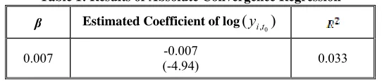
Table 1 shows the estimation results of equation (2) for 22 MENA countries1 from 1970- 2003. It includes the estimated value of the coefficient of independent variable with its t- value in parentheses, the corresponding derived value of β and the value of R2. The estimated positive value of β, derived from the negative coefficient of log( )
0
,t i
y , which is statistically significant, demonstrates existence of absolute β convergence.The relatively low value of R2 is not unusual in such cross-sectional equation estimates. Such values in general can reflect the significance of omitted factors. In addition, structural heterogeneity and differences in initial conditions of 22 MENA countries may determine different steady states for these countries.
Table 1: Results of Absolute Convergence Regression
β Estimated Coefficient of log( )
0
,t i y
0.007 -0.007
(-4.94) 0.033
This table presents the results of linear regression model for absolute convergence, the positive sign of β support existence of absolute convergence with low speed.
Equation (10) summarizes these results, Where gy is the annual growth rate of country i at time t:
)
log(
).
1
(
115
.
0
0.007 , 1 − −∧
−
−
=
itit
e
y
gy
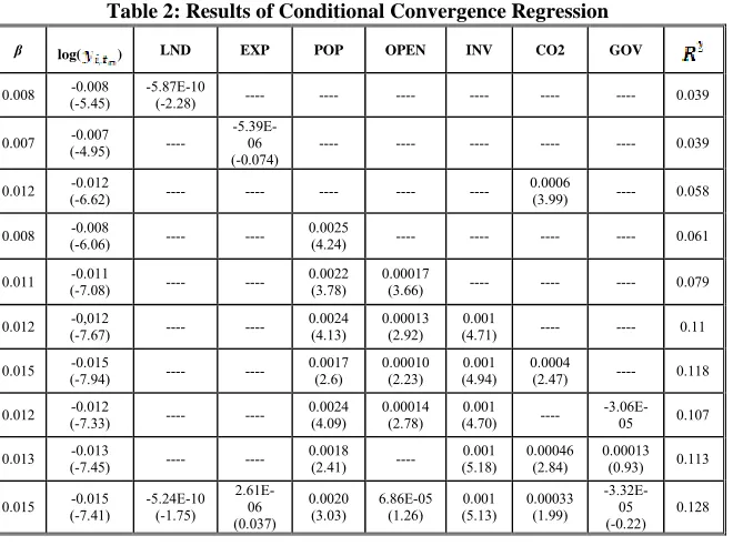
(10)Accordingly, after we condition on steady state as described in equation (3) by adding different independent variables, we estimate the conditional convergence in Table 2. Variables added linearly to the original model include arable land (LND), life expectancy (EXP), annual growth rate of population (POP), openness in constant price (OPEN), investment share of real GDP (INV), metric tons per capita of CO2 emissions (CO2) and percentage of government expenditure from GDP (GOV).
Table 2: Results of Conditional Convergence Regression
β log( ) LND EXP POP OPEN INV CO2 GOV
0.008 (-5.45) -0.008 -5.87E-10 (-2.28) ---- ---- ---- ---- ---- ---- 0.039
0.007 (-4.95) -0.007 ---- -5.39E-06
(-0.074) ---- ---- ---- ---- ---- 0.039
0.012 (-6.62) -0.012 ---- ---- ---- ---- ---- 0.0006 (3.99) ---- 0.058
0.008 (-6.06) -0.008 ---- ---- 0.0025 (4.24) ---- ---- ---- ---- 0.061
0.011 (-7.08) -0.011 ---- ---- 0.0022 (3.78) 0.00017 (3.66) ---- ---- ---- 0.079
0.012 (-7.67) -0,012 ---- ---- 0.0024 (4.13) 0.00013 (2.92) (4.71) 0.001 ---- ---- 0.11
0.015 (-7.94) -0.015 ---- ---- 0.0017 (2.6) 0.00010 (2.23) (4.94) 0.001 0.0004 (2.47) ---- 0.118
0.012 (-7.33) -0.012 ---- ---- 0.0024 (4.09) 0.00014 (2.78) (4.70) 0.001 ---- -3.06E-05 0.107
0.013 (-7.45) -0.013 ---- ---- 0.0018 (2.41) ---- (5.18) 0.001 0.00046 (2.84) 0.00013 (0.93) 0.113
0.015 (-7.41) -0.015 -5.24E-10 (-1.75) 2.61E-06 (0.037)
0.0020 (3.03)
6.86E-05 (1.26)
0.001 (5.13)
0.00033 (1.99)
-3.32E-05
(-0.22) 0.128
This table presents the results of linear regression model for conditional convergence, the positive sign of β support existence of absolute convergence. T-statistics in parentheses show significance of conditional convergence.
As the results show, additional variables improve the explanatory power of the model very slightly, and in all presented models of Table 2 coefficient of log( )
0
,t i
y is statistically significant with the negative sign. Additional variables like arable land, life expectancy, ratio of government expenditure to GDP are statistically insignificant and do not add to the model. Openness and CO2 emissions in some models are insignificant. Accordingly, the best model is:
INV OPEN
POP t
i y e
it
gy∧ =0.124−(1− −0.012).log( , −1)+0.0024 +0.00013 +0.001
(11)
We then use nonparametric ANN approach to make the estimation more accurate. A neural network uses three samples of data.
Validation sample which is used f o r measuring network generalization and halting training when generalization stops improving and testing sample that has no effect on training and so provide an independent measure of network performance during and after training. The most important challenge of neural network performance is related to its architecture. Usual way for designing a suitable network is trial and error.
We examined more than 50 different neural networks to find the best network’s architecture empirically and used training, validation and testing subsamples with 70%, 15%, 15% -70%, 20%,10% -80%, 10%, 10% and 60%, 20%, 20% which are more general orders for ANN algorithm and found 70%, 15%, 15% subsample is the best. Therefore, 1970-93 is the training sample, 1993-1998 is the validation sample and 1998- 2003 is the testing sample. According to equations (4) to (9) we used BPN feed-forward network model as follow:
⎟ ⎟ ⎠ ⎞ ⎜ ⎜ ⎝ ⎛ + + = ⎟ ⎟ ⎠ ⎞ ⎜ ⎜ ⎝ ⎛ − − =
−
∑
1 ( *log( )0 1
, ,0 , 1)
* 1 1 log t i k y k k k t i it e y y ω
γ
γ
(12)And ELMAN recurrent network model:
⎟⎟ ⎠ ⎞ ⎜⎜ ⎝ ⎛ + + = ⎟ ⎟ ⎠ ⎞ ⎜ ⎜ ⎝ ⎛ − =
−
∑
nitk k k t i it e y y , * 1 1 log 1 0 1 ,
γ
γ
(13)∑
∑
= − = − + + = * * 1 1 1 , 1 , , 0 ,, *log( )
i i k k t k k t i i k k t
k y n
n
ω
ω
φ
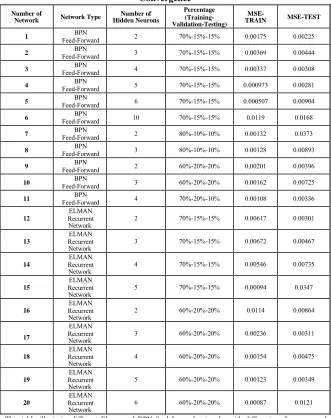
(14)Table 3: Results of Different Artificial Neural Networks for Absolute Convergence
Number of
Network Network Type
Number of Hidden Neurons
Percentage (Training-Validation-Testing)
MSE-TRAIN MSE-TEST
1 Feed-Forward BPN 2 70%-15%-15% 0.00175 0.00225
2 Feed-Forward BPN 3 70%-15%-15% 0.00369 0.00444
3 Feed-Forward BPN 4 70%-15%-15% 0.00337 0.00308
4 Feed-Forward BPN 5 70%-15%-15% 0.000973 0.00281
5 Feed-Forward BPN 6 70%-15%-15% 0.000507 0.00904
6 Feed-Forward BPN 10 70%-15%-15% 0.0119 0.0168
7 Feed-Forward BPN 2 80%-10%-10% 0.00132 0.0373
8 Feed-Forward BPN 3 80%-10%-10% 0.00128 0.00893
9 Feed-Forward BPN 2 60%-20%-20% 0,00201 0.00396
10 Feed-Forward BPN 3 60%-20%-20% 0.00162 0.00725
11 Feed-Forward BPN 4 70%-20%-10% 0.00108 0.00336
12
ELMAN Recurrent
Network 2 70%-15%-15% 0.00617 0.00301
13
ELMAN Recurrent
Network 3 70%-15%-15% 0.00672 0.00467
14
ELMAN Recurrent
Network 4 70%-15%-15% 0.00546 0.00735
15
ELMAN Recurrent
Network 5 70%-15%-15% 0.00094 0.0347
16
ELMAN Recurrent
Network 2 60%-20%-20% 0.0114 0.00864
17
ELMAN Recurrent
Network 3 60%-20%-20% 0.00236 0.00311
18
ELMAN Recurrent
Network 4 60%-20%-20% 0.00154 0.00475
19
ELMAN Recurrent
Network 5 60%-20%-20% 0.00123 0.00349
20
ELMAN Recurrent
Network 6 60%-20%-20% 0.00087 0.0121
This table illustrates different Elman and BPN feed-forward networks with different performance and different errors.MSE measurement for
testing sample shows that the best capable networks are the first and fourth one.
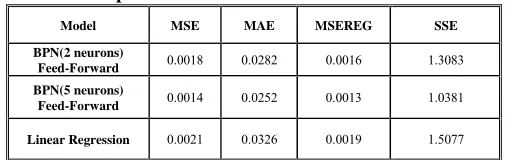
performance will be chosen according to MSE of testing sample. The ability of the network to estimate accurately the annual rates of growth, which is our dependent variable, based on unused values of the independent variable in training indicates that it has sufficiently captured the underlying relationship and the networks perform well with new data from testing sample, which are fed to networks after training. Despite the dynamic of Elman recurrent networks, the first and fourth neural network models BPN, feed-forward with two and five hidden neurons are those networks that minimize MSE in testing sample and can produce estimations that are more accurate. Table 4 presents the performance of these networks in total sample in comparison with linear regression model more specifically.
Table 4: Comparison of ANN and Linear Model Performance
Model MSE MAE MSEREG SSE
BPN(2 neurons)
Feed-Forward 0.0018 0.0282 0.0016 1.3083
BPN(5 neurons)
Feed-Forward 0.0014 0.0252 0.0013 1.0381
Linear Regression 0.0021 0.0326 0.0019 1.5077
This table shows the performance of artificial neural networks and linear regression model with different measurement of their errors. It supports that ANN is more accurate.
As the results show, mean squared error (MSE), mean absolute error (MAE), mean squared error with regularization (MSEREG)1 and sum
1- Msereg is a network performance function that measures network performance as the weight sum of two factors: the mean squared error and the mean squared weight and bias values. The formula of Msereg is shown below:
Where γ is the performance ratio (the ratio of importance between errors and weights), and
∑ = = N
i ei N MSN
1 2 ) ( 1
∑ = = N
i wj n MSN
1 2 1
squared error (SSE) of BPN feed- forward neural networks are less than those of linear regression model. Hence, neural network is a more capable and more accurate model than linear regression model. As the results show, ANN with five hidden neurons is the best one and is chosen.
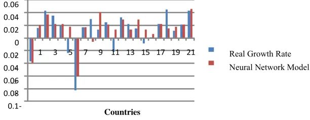
We report values of R2 for ANNs, but the definition of R2 breaks down as we move away from traditional regression. For the best vision about the ANN performance, Figure 4 shows in-sample evaluation of it. It illustrates a randomly selected year, 1990, which has been used during training in comparison with the real data.As can be observed, the network performs well in estimation of growth rates.
Figure 4: In-Sample Performance of ANN for 1990
This figure shows In-Sample performance of artificial neural networks for 1990, randomly selected, for 22 MENA countries.
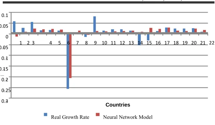
Figure 5 plots out-of-sample performance of ANN. It shows growth rates of 22 MENA countries in comparison with the estimated growth rates of selected neural network model for the year 2003, which is last period in testing sample. It is expected that estimation is less accurate than in-sample but still it is appropriate.
‐
0.1
‐
0.08
‐
0.06
‐
0.04
‐
0.02 0 0.02 0.04 0.06
1 3 5 7 9 11 13 15 17 19 21
Growth Rate
Countries
Figure 5: Out-of-Sample Performance of ANN for 2003
This figure illustrates Out-of-Sample performance of ANN. It compares the neural network estimations with real data of growth rate of MENA countries in 2003.
All of these figures and tables prove the capability of neural networks for studying income convergence and capturing the movement of different countries growth rates. Artificial neural networks also, can be used for analyzing unconditional income convergence.As Table 2 presents, additional variables like POP, INV and OPEN are statistically significant and we can use them in ANN models to study conditional convergence. Table 5 summarizes some of ANN models for conditional convergence.
Table 5: Results of Different Artificial Neural Networks for Conditional Convergence
Number of
Network Network Type Hidden Neurons Number of (Training-Validation-Testing)Percentage MSE-TRAIN MSE-TEST
1 Feed-Forward BPN 3 70%-15%-15% 0.00516 0.0108
2 Feed-Forward BPN 4 80%-10%-10% 0.00158 0.00372
3 Feed-Forward BPN 5 85%-10%-5% 0.000581 0.00226
4 Recurrent Network ELMAN 2 70%-15%-15% 0.00293 0.00268
5 Recurrent Network ELMAN 3 80%-10%-10% 0.00686 0.00573
6 Recurrent Network ELMAN 5 60%-20%20% 0.00115 0.00856
This table illustrates different Elman and BPN feed-forward networks with different performance and different errors for conditional convergence.
‐
0.3
‐
0.25
‐
0.2
‐
0.15
‐
0.1
‐
0.05 0 0.05 0.1
1 2 3 4 5 6 7 8 9 10 11 12 13 14 15 16 17 18 19 20 21 22
Growth Rate
Countries
‐0.06
‐0.04
‐0.02 0 0.02 0.04 0.06 0.08 0.1
1 2 3 4 5 6 7 8 9 10 11 12 13 14 15 16 17 18 19 20 21 22
Gr
o
w
th
Ra
te
Countries
Real Growth Rate Neural Network Model
Model 3, with 5 hidden neurons is the best and more accurate network according to MSE of both testing and training samples. Like absolute convergence we can compare the performance of OLS and ANN models. Table 6 presents the results:
Table 6: Comparison of ANN and Linear Model Performance
Model MSE MAE MSEREG SSE
BPN(5 neurons)
Feed-Forward 0.000933 0.021 0.000839 0.677 Linear Regression 0.0019 0.0319 0.0017 1.342 This table shows the performance of artificial neural networks and linear regression model with different measurement of their errors for conditional convergence. It supports that ANN is more accurate.
Again, the performance of neural network is better than linear regression model. Like unconditional convergence, in-sample and out-of-sample performance of 22 MENA countries are presented in Figure 6 and Figure 7.
Figure 6: In-Sample Performance of ANN for 1987
‐0.3
‐0.25
‐0.2
‐0.15
‐0.1
‐0.05 0 0.05 0.1
1 2 3 4 5 6 7 8 9 10 11 12 13 14 15 16 17 18 19 20 21 22
G
ro
w
th
R
a
te
Counries
Real Growth Rate Neural Network Model
Figure 7: Out-of-Sample Performance of ANN for 2003
This figure illustrates Out-of-Sample performance of ANN. It compares the neural network estimations with real data of growth rate of MENA cuntries in 2003.
gain, like in absolute convergence, the results are accurate. Additional variables like OPEN, INV and POP make the out-of-sample performance of the model more accurate than in figure 5 but in both figures ANN performs so well.
Conclusions
As our results show, absolute convergence exists for 22 MENA countries across the world in studied period of 1970-2003. It means that our analysis supports tendency of poor economies to grow faster than rich ones across the MENA countries. In addition, after conditioning some different variables like openness, annual growth rate of population, investment, etc. we conclude that conditional β convergence is statistically significant in all of estimated models but the speed of convergence is low.
Elman recurrent networks, the BPN, feed-forward neural network model with five hidden neurons is the one, which can produce estimations that are more accurate.
The most important point of this study is that although we compare neural network’s accuracy with regression model and conclude neural networks are more capable, we used artificial neural networks as the complement algorithm of OLS method, not as the alternative or substitute approach.
We recommend as Barro and Sala-i-Martin (2004) did, that future studies try to survey income convergence, by both regression method and ANN algorithm for more similar economies, like regions of a country or countries of a trading block. In addition, one can use artificial neural networks with other approaches like time series or panel data.
References
1- Abramovitz, M. (1986). “Catching up, forging ahead and falling behind”. Journal of Economic History 46, 385–406.
2- Barro, R. & Sala-i-Martin, X (1990). "Economic Growth and Convergence across the United States", Working Paper no.3419, NBER, Cambridge,.Massachusetts. Barro, R. & Sala-i-Martin, X (1992). "Convergence", Journal of Political Economy, 100, 223-151.
3- Barro, R. & Sala-i-Martin, X (2004). Economic Growth. Cambridge Ma: MIT Press. Baumol,W. (1986). “Productivity growth, convergence, and welfare:What the long-run data show”. American Economic Review 76 (5), 1072–1085.
4- Benhabib, J and Spiegel, M. M., (1997), “Cross-Country Growth Regressions”, Working Paper 97-20, CV Starr Center, New York University. 5- Bernard, A., Durlauf, S. (1995). “Convergence in international output”.
Journal of Applied Econometrics 10 (2), 97–108.
6- Bernard, A., Durlauf, S. (1996). “Interpreting tests of the convergence hypothesis”.Journal of Econometrics 71 (1–2), 161–173.
9- Caselli, F., Esquivel, G., Lefort, F. (1996). “Reopening the convergence debate: a new look at cross country growth empirics”. Journal of Economic Growth 1 (3), 363–389. DeLong, J.B. (1988). “Productivity growth, convergence, and welfare: Comment”. American Economic Review
78 (5), 1138–1154.
10- Durlauf, S. N. & Quah, D.T (1998). “The New Empirics of Economic Growth”, the University of Wisconsin, Madison and LSE.
11- Durlauf, S. N. & Johnson, P.A & Temple, J.R (2005). “Growth Econometric” Handbook of Economic Growth, Vol 1(a). p. 561-660.
12- Evans, P. (1998). “Using panel data to evaluate growth theories”.
International EconomicReview 39 (2), 295–306.
13- Fiaschi, D. & Lavezzi, A.M (2007). “Productivity Polarization and Sectoral Dynamic.in European Regions”, Journal of Macroeconomics, 29, 612–637.
14- Islam, N. (2003). “What Have We Learned from the Convergence Debate?”, Journal ofEconomic Surveys ,17, 309–362.
15- Islam, N. (1995). “Growth empirics: A panel data approach”. Quarterly Journal ofEconomics 110 (4), 1127–1170.
16- Islam, N. & Sakamoto, H. (2006). “Convergence Across Chinese Provinces: An.Analysis Using Markov Transition Matrix” China Economic Review.
17- Jones, L., Manuelli, R. (1990). “A convex model of equilibrium growth: Theory and policy implications”. Journal of Political Economy 98 (5), 1008–1038.
18- Kelly, M. (1992). “On endogenous growth with productivity shocks”.
Journal of Monetary Economics 30 (1), 47–56.
19- Koopmans, T.C. (1956). "The Klein-Goldberger Forecasts for 1951, 1952 and 1954, Compared with Naive-Model Forecasts," Cowles Foundation Discussion Papers 12, Cowles Foundation, Yale University. 20- Lee, K.& Pesaran, M. H. & Smith, R. (1997). “Growth and Convergence in a Multi- Country Empirical Stochastic Solow Model”,
Journal of Applied Econometrics, 12,357-392.
21- Lucas, R. (1988). “On the mechanics of economic development”.
22- Mankiw, N.G., Romer, D.,Weil, D.N. (1992). “A contribution to the empirics of economic growth”. Quarterly Journal of Economics 107 (2), 407–437.
23- McNelis, P.D., (2005). “Neural Networks in Finance: Gaining Predictive Edge in the Market.” Elsevier Academic Press. 118-224.
24- Nahar, S. & Inder, B. (2002), “Testing Convergence in Economic Growth for OECD Countries”, Applied Economics, 34, 2011-2022.
25- Nerlove, M. (1996). “Properties of alternative estimators of dynamic panel models: An empirical analysis of cross-country data for the study of economic growth”. In: Hsiao, C. (Ed.), Analysis of Panels and Limited Dependent Variable Models: In Honor of G.S. Maddala. Cambridge University Press, Cambridge.
26- Pesaran, M.H. (2004a). “A Pair-Wise Approach to Testing for Output and Growth Convergence”. Mimeo, University of Cambridge.
27- Pesaran, M.H. (2004b). “General Diagnostic Tests for Cross-Section Dependence in Panels”.Mimeo, University of Cambridge.
28- Papadas .C.T , Efstratoglou.S (2004). “Estimation of Regional Economic Convergence Equations Using Artificial Neural Networks with Cross Section Data”. Greece. Agricultural University of Athens.
29- Quah, D. (1993a). “Galton’s fallacy and tests of the convergence hypothesis”, Scandinavian Journal of Economics 95, 427–443.
30- Quah, D. (1993b). “Empirical cross-section dynamics in economic growth”. European Economic Review 37 (2–3), 426–434.
31- Quah, D. (1996a). “Twin peaks: growth and convergence in models of distribution dynamics”. Economic Journal106 (437), 1045–1055.
32- Quah, D. (1996b). “Empirics for economic growth and convergence”.
European Economic Review 40 (6), 1353–1375.
33- Quah, D. (1996c). “Convergence empirics across economies with (some) capital mobility”. Journal of Economic Growth 1 (1), 95–124.
34- Quah, D. (1997). “Empirics for growth and distribution: Stratification, polarization, and convergence clubs”. Journal of Economic Growth 2 (1), 27–59.
36- Quah, D. and Durlauf, S. N., (2004). “Handbook of Macroeconomics” 4 (2), 238- 256. Ramsey F.P. (1928). "A mathematical theory of saving".
Economic Journal, vol. 38, no.152, 1928, pages 543–559.
37- Romer, P. (1986). “Increasing returns and long-run growth”. Journal of Political Economy 94 (5), 1002–1037.
38- Schalkoff, R. J. (1997). “Artificial Neural Networks”. Mcgraw-Hill Press.25-44.
39- Solow, R. (1956). “A Contribution to the Theory of Economic Growth”, Quarterly Journal of Economics LXX, 65-94.
40- Summers, R. & Heston, A. (2006). “The PennWorld Table (Mark 6.2): An expanded set of international comparisons, 1950–2004”. Quarterly Journal of Economics 106 (2), 327–368.
41- Swan, T. (1956). “Economic growth and capital accumulation”.
Economic Record 32, 334–361.
42- W.D.I (2008). “World Development Indicator” World Bank Press. 43- Warner.B, Misra.M (1996). “Understanding Neural Networks as Statistical Tools”