Application of AERMOD to local scale diffusion and dispersion
modeling of air pollutants from cement factory stacks
(Case study: Abyek Cement Factory)
Noorpoor, A.1* and Rahman, H.2
1
Associate Professor, Graduate Faculty of Environmental, University of Tehran, Tehran, Iran
2
MSc Student of Environmental Engineering, University of Tehran, Tehran, Iran
Received: 19 Apr. 2015 Accepted: 24 Jun. 2015
Abstract: Today, the cement industry is one of the major air polluting industries in the
world. Hence, in this study, owing to the importance and role of contaminants from the plant, an appraisal of the emission contributions in addition to other factors have been discussed. There are several reasons behind the importance of modeling air pollutants. First, the assessment of standards for air pollution, and the fact that the measurement points are limited. Furthermore, in all industrial areas, measurement and installation of assessment and monitoring stations are not feasible. The AERMOD model is a dispersion steady state model which is utilized to determine the concentration of various pollutants in different areas from urban and rural, flat and rough, shallow diffusion in height, from standpoint and different shallow sources. In this model, it is assumed that the dispersion of concentration in Stable Boundary Layer (SBL) in two horizontal and vertical directions are similar to that of horizontal within Gaussian convectional boundary layer (CBL). With regard to assessment of the parameters and pollutants of stack outlet, the amount of particulate matter was measured as the most important pollutant in the region. Then, via dispersion and diffusion modeling of pollution (AERMOD) along with environmental measurements, the nature of dispersion of this pollutant in the analysis of the surrounding areas was verified. According to the presented results, the highest level of concentration for particulate matters in all areas affected by cement factory amounts to 43.68 (µg/m3) which occurred at a distance of 1500 m in the east direction and 2100 m in the north direction.
Keywords: air pollution, cement industry, diffusion and dispersion modeling, particulate matter.
INTRODUCTION
Today, the industrial complex which has big size of combustion chamber produce air pollutants, and have to be considered. Abyek cement industry in Iran has the biggest combustion chamber in the middle-east with a capacity of 8000 ton clinker per day. The local air quality has been an issue of social concern because of rising
* Corresponding author Email: [email protected]
Most of these studies were conducted in developed countries, and only a small number of studies have been conducted in Asia's developing countries (Health Effects Institute, 2004; Chen et al., 2010). One of the major pollutants in the borderlands is particulate matter (PM), which is categorized into particles with aerodynamic diameter less than 10 mm (PM10) and those less than 2.5 mm (PM2.5 or fine PM). It is the US EPA’s regulatory PM10 standard that is frequently violated in the border towns, with reported violations of the PM2.5 standard being far fewer (Choi et al., 2006). Hence, in this study, owing to the importance and role of contaminants from the plant, appraisal of the emissions contribution in addition to other factors have been discussed. For this purpose, in the first place, the flow parameters and the particulate matter from stack outlet were measured using appropriate equipment. Then, by applying the AERMOD software, diffusion and dispersion of particulate matter in the surrounding area was modeled.
Air quality largely influences the ecology, environment and public health in a region. In recent years, several research efforts have been made to developair quality prediction models. Atmospheric dispersion models are used to predict the ground level concentration of the air pollutants around the sources (Cimorelli et al., 2005; EPA, 2005; Kesarkar et al., 2007; Bhaskar et al., 2008; Singh et al., 2012). Air pollution is of particular concern in urban and industrial areas where significant emissions coupled with unfavorable meteorology may lead to pollutant accumulation and long-term exposure. In such contexts, an integrated approach of Air Quality Management (AQM) is needed. Long- term monitoring campaigns are associated with high costs and often lack sufficient spatial density to adequately characterize ambient air quality (Prabha and Singh, 2006), particularly in
areas where air quality exhibits large spatial and temporal variations due to complex meteorology and terrain, variable land use, and shoreline fumigation (Ghannam and El-Fadel, 2013).
There are several reasons behind the importance of modeling air pollutants. First, the assessment of standards for air pollution and the measurement points are limited. Furthermore, in all industrial areas, measurement and installation of assessment and monitoring stations are not feasible. It would also be possible, by means of measurement, to assess the modeling results and reduce its error and uncertainty (Zou et al., 2011). Dispersion modelling uses mathematical equations, describing the atmosphere, dispersion of chemical and physical processes within the plume, to calculate concentrations at various locations.
The American Meteorological Society and EPA developed the AERMOD modeling system (Cimorelli et al., 2004). Treatment of both surface and elevated point sources, area sources, and volume sources in a simple or complex terrain model domain are addressed in the model. It was intended as a replacement of the Industrial Source Complex Version 3 (ISC3) model. Currently, AERMOD is the EPA’s preferred model for regulatory compliance and demonstration for criteria pollutants in the near field (<50 km) (Rood, 2014).
Air dispersion modeling calculates the movement of pollutants that are in the air using mathematical models that consider emission quantities, meteorology, topographical factors, and chemical and physical processes within the atmosphere over time and space, in order to calculate concentrations of air pollutants at different ‘receptors’ (researcher-defined locations for concentration calculations). If sufficient data exist and are accessible for pollution sources and environmental conditions, air dispersion modeling has the potential to provide a more accurate assessment of possible exposure without the need for extensive monitoring networks (Dent et al., 1998; Hodgson et al., 2007; Jerrett et al., 2005; Maroko, 2012).
Air pollution modelling is performed by finding out the amount of dispersion from sources, concentration in sampling station, meteorology and topography data, the kind of ground usage. In modeling, there is a dynamic relationship between sources of dispersion and concentration which ultimately leads to dispersion of pollutants in places with no assessment station.
Because of the entering of suspended particles from the West of the country to the study area, in order to determine and evaluate the factory's share of total available particles, the amount of particles in the atmosphere is measured at four points around the plant using the SKC pump. By subtracting the measured amount of particles resulting from modeling, from measured ones using the SKC pump, Abyek cement factory's share percent, compared to other sources of pollution in the region, can be estimated.
MATERIALS AND METHODS
Of course, the detail and quality of the input requirements depend on the sophistication of the model used. Older dispersion models, i.e. simple Gaussian plume models, are based on the use of the Pasquill-Gifford-Turner stability classes
for the characterization of the vertical and lateral dispersion (EPA, 1995). Instead, the new generation of short-range dispersion models, including more complex Gaussian plume models such as ISC3, AERMOD and ADMS, uses the Monin-Obukhov similarity to describe the mean and turbulence structure in the surface boundary layer. The ground-level concentration is generally expressed in terms of specific variables, such as the surface friction velocity and the Monin-Obukhov length, which contain information on the turbulence and the mean wind that govern dispersion (Vankatram, 2004; Capelli et al., 2013).
This division of mass is implemented based on the connection between the height of critical stream line and the vertical dispersion of concentration in each recipient.
AERMOD predict the most stable condition and the lowest mixing height, being the emission above the mixing height. For the rest of the simulated period, a lower concentration far away from the source at the ground level was observed. This is because the instability of the atmosphere was increasing and the vertical spread is higher, distributing the contaminant along the whole PBL at a higher height (Caputo et al., 2003).
In this research, in order to model the diffusion and dispersion of pollutants, the AERMOD model was employed. The AERMOD model is a stack in a stable condition which explains the dispersion of air based on the structure of boundary layer
and turbulence in an acceptable scale. AERMOD is a permanent dispensational state which is used to determine the concentration of various pollutants in urban and rural areas, shallow diffusion and in the height of standpoint and shallow sources. It is mainly proposed to assimilate dispersion of pollutants in limit of 50 Km.
Abyek cement factory is located in the east of Alborz Province in Iran. It is in latitude 36 degrees 1 minute and longitude 50 degrees 35 minutes. The plant’s elevation is 1440 m above sea level. Four cities namely Hiv, Hashtgerd, Nazarabad, Abyek are around this cement factory and the mean distance of each of them from Abyek cement factory respectively is equal to 5,9, 6, and 5 Km. The total human population of this area is more than 250,000. Figure 1 shows the location of the factory in Iran, Alborz Province.
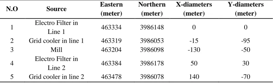
To achieve the research objectives, primarily the output suspended particulates from the cement factory’s stacks should be measured by sampling. Thus, output gas speed, temperature and pressure were measured by applying the device KIMO and suspended particulate matter were assessed by using WESTECH. Table 1
shows the location of stacks in the Universal Transverse Mercator (UTM) coordinate system, Local coordinate system and also the line 1 electro filter of the cement factory were considered at the origin and the property of other recipients relative to it were determined.
Table 1. Location of stacks in Universal Transverse Mercator (UTM) coordinate system and Local coordinate
system
N.O Source Eastern
(meter)
Northern (meter)
X-diameters (meter)
Y-diameters (meter)
1 Electro Filter in
Line 1 463334 3986148 0 0
2 Grid cooler in line 1 463319 3986053 -15 -95
3 Mill 463204 3986098 -130 -50
4 Electro Filter in
Line 2 463384 3986178 50 30
5 Grid cooler in line 2 463478 3986078 140 -70
Measurements from fixed monitoring stations (FMS) have been commonly used as surrogates for personal exposure levels to represent community exposure to pollutants. Exposure estimates obtained from FMSs have been the basis of air quality guidelines and policy (Kaur et al., 2005).
AERMOD uses a meteorological preprocessor called AERMET to characterise the atmospheric conditions in the Planetary Boundary Layer, and a terrain preprocessor called AERMAP to characterize terrain elevation and prepare source/receptor heights for pollutant dispersion (Misra et al., 2013). This model, in addition to the main AERMOD processor is made of a topographical preprocessor called AERMAP. The AERMAP preprocessor analyzes the regional topographical information. Ultimately, the model perform its final sources using results of this preprocessor and the complementary information regarding the diffusion sources and the recipient net.
The ground level data included are: topography, mean sea level pressure, local pressure, temperature, friction velocity,
the emission source: in cases of complex terrain, the meteorological station shall be located in the same valley or in a position as to be representative of the wind conditions of the considered emission. This is particularly true for the wind speed and wind direction data. The data registration frequency and the extension of the simulation time domain may depend on the simulation purposes (Capelli et al., 2013). All necessary ground-level data were obtained from the nearest National Weather Service (NWS) station located in Hashtgerd City, code 99396, located 15 km from the original study site. Due to the lack of available data on Abyek, Hashtgerd Station data was used as well. On the basis of meteorological data, two statistical periods have been performed for the first and third quarters of 2013 (O’Shaughnessy and Altmaier, 2011).
For any atmospheric condition, AERMET can calculate the mixing height or use the value given by input. For stable atmospheric condition, if the user introduces the mentioned value, it is assigned to the mechanical mixing height, otherwise it is internally calculated. Under unstable condition, the code chooses the maximum between the value given by input and the mechanical mixing height calculated internally (Capelli et al., 2013). The AERMET processor is designed in such a way which makes it feasible to define all the existing meteorological information within the onsite and use them for processing. Therefore, in this project precipitation amount, sky cover, station pressure, sea level pressure as surface parameters, also dew-point temperature, wind direction, and relative humidity were considered as profile parameters.
The settings and parameters for AERMOD were determined and processed with those (e.g. albedo, bowen ratio, and surface roughness) described in our earlierwork (Zou et al., 2010). After these preparations, the AERMOD model was run
at daily and annual temporal scales, for simulating the PM concentrations at each receptor from different emission sources (Zou et al., 2010). As it has been mentioned, in order to perform its calculations (AERMET) needs three surface parameters from the studied region, namely Bowen ratio, Albedo coefficient and the roughness length of surface. The Albedo coefficient is sunlight radiation which is reflected to space without absorption by surface. Its amounts varies from 0.1% for woods with dense trees to 0.9% for soft snow. Bowen ratio is an index to determine the moisture ratio of sensible heat flux to latent heat flux. During the day, its amount varies from 1% for water surface to 10 for desert surface. The length of surface roughness is related to the wind stream and the height of surface barriers. In fact, it is a height in which, the average of the horizontal velocity of wind reach to zero. The amount of these parameters range from the limit of less than 0.001 m for stagnant surface water to more than 1 m for wood surfaces and urban regions.
PBL height depends on the strength of both convective mixing of air masses generated by the solar heating of the Earth’s surface and by mechanical mixing due to the interaction between wind and surface roughness (Oke, 1987; Stull, 1988). In sunny days and when mechanical mixing is not relevant (i.e., low wind speed conditions), PBL exhibits a typical diel (24 h) cycle characterized by low nocturnal levels and elevated daytime heights. During the night, when mechanical turbulence is present, PBL heights can rise significantly over the typical nighttime levels (Morselli et al., 2012).
RESULTS
Air quality model can be an adequate tool for future air quality prediction, also for atmospheric observations supporting emission control and strategy responders. The model of AERMOD is used as a tool for the analysis of particulate matter emissions from an industrial complex, as a part of environmental impact assessment. Both variability and uncertainty affect Gaussian modeling results. Variability in the Gaussian model, results primarily through meteorology and emission rates, because weather conditions and processing rates vary over time. We believe uncertainty in Gaussian models can be categorized into three components: input uncertainty, parameter uncertainty, and conceptual uncertainty. The AERMOD model was applied as a tool for the analysis of particulate matter (PM) emissions from a cement complex, as a part of the environmental impact assessment. The dispersion of PM from four cement plants within the selected cement complex was investigated both by measurement and AERMOD simulation in dry and wet seasons. Simulated values of NO2
emissions were compared with those obtained during a 7-day continuous measurement campaign at 4 receptors.
The AERMOD model requires special information for each kind of pollutant and sources. For used sources of this research which are considered as standpoint sources, the same information is required such as the rate of pollutant dispersion, the height of pollutant released from the
ground surface, temperature and velocity of outlet gas from the sources, also the internal diameter of stack and exit place which were determined for each of the sources. In addition, it is necessary to specify the position of sources in relation to each other. To do this, it is possible to determine the position of stacks in the Universal Transverse Mercator (UTM), relative to an arbitrary origin.
In this research, the line 1 electro filter is considered as the origin and property of other sources relative to it is determined and introduced and also the recipients in Cartesian position within limit of 35*35 Km², which web distance on 100 meters (351 web line) in each, the two directions of X,Y are defined. Arrangement of recipients relative to a selective origin, namely line 1 electro filter. It is necessary to mention that in this case study, assimilation is performed for the recipients situated on the ground surface.
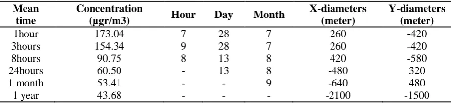
Table 2 shows the maximum concentration for mean time at 1hour, 3hours, 8hours, 24hours, 1month and 1 year.
Figure 2 shows the dispersion of TSP pollutant for all the plant sources in satellite view. Also, Figure 3 shows the seasonal (on the basis of meteorological data of the second quarter of 2013) dispersion of TSP pollutant.
Figure 4 show the dispersion of TSP pollutant for all of the plant sources in satellite view, also, Figure 5 shows the seasonal (on the basis of meteorological data of third quarter of 2013) dispersion of TSP pollutant.
Table 2. Maximum concentration of TSP for Separate mean times
Mean time
Concentration
(µgr/m3) Hour Day Month
X-diameters (meter)
Y-diameters (meter)
1hour 173.04 7 28 7 260 -420
3hours 154.34 9 28 7 260 -420
8hours 90.75 8 13 8 420 -580
24hours 60.50 - 13 8 -480 320
1 month 53.41 - - 9 -640 480
Fig. 2. Dispersion of TSP pollutants for all the plant sources Fig. 3. Seasonal dispersion of TSP Pollutants
Fig. 4. Dispersion of TSP pollutants for all of the plant sources Fig. 5. Seasonal dispersion of TSP Pollutants
The Figures show that the urban areas of Nazarabad and Abyek are less affected by the sources of the particulate matter exited from the cement factory source. The Hiv and Hashtgerd areas due to dominant wind and the movement of pollutant in the direction from South-west to North- east, are more affected by pollution sources.
The previous concentration in various temporal local conditions as it has been mentioned earlier, in this research, the nature of pollutant dispersion for particulate matter dispensed by Abyek
cement factory in limit of 35*35 Km² was carried out. The average time period of 1, 3, 8, 24 h and the statistical one-month and one-year period as well as the altitude of ground surface were considered.
for the maximum-hourly average concentration (Rood, 2014). Sampling was carried out in order to analyze and verify the modeling for the dispersion of
particulate matter in the surrounding area. Table 3 shows the concentration of TSP pollutant in the surroundings of Abyek cement factory.
Table 3. The concentration of TSP pollutant in surroundings of Abyek cement factory
Sampling Point Distance(meter) Concentration(µgr/m3)
Point 1 (Abyek) 6200 282.2
Point 2 (Hiv) 4600 354.8
Point 3 (Nazarabad) 5300 235.7
Point 4 (Hashtgerd) 9800 268.8
CONCLUSION
The model was defined and performed with respect to all data centered around the Abyek cement industry. The results of these modeling were transferred to Google Earth software via the Arc GIS software and final results were observed. In this research, the model was assessed for three states. The first state concern assessment of the amount of pollution steamed from the factory's first line, and second line, respectively. The third state was carried out for all the factory stack outlets, in order to separately assess facts separately.
The maximum concentration in unstable conditions in the boundary layer of the atmosphere, in larger extent of concentration occurred in stable condition, and the maximum amounts of concentration occurred in farther distance from the similar but stable conditions in the boundary layer of the atmosphere. The findings indicate that there is a reverse relationship between concentration and wind velocity in Gaussian model. Moreover, the concentration depends on the emission factors, the effective height of plume rise, atmospheric conditions, wind velocity and the meteorological parameters have an important role in emission of air pollutants.
Comparison of results in a functional state (enabled simultaneously for all sources) is presented in Table 2, by proposed limit values for particulate emissions, shows that even though all the plant sources are active, the maximum
concentration for mean time at 24 h and 1 year are much lower than the clean air standards.
As the satellite image (Fig. 2) shows some areas such as Nazarabd and Abyek, which are less affected by output of particulate emissions from cement plants. Although in comparison with other areas, Ivan district is more affected by pollution from these sources, it does not meet the limit proposed by the Environmental Protection Agency.
According to the presented results, the maximum concentration of particulates originating from Abyek cement plant in all points is equal to 43.68 microgram per cubic meter and occurred at a distance of 2100 m and 1500 m in the south-east direction. Furthermore, the model was implemented according to the NIOSH0500 standard and for the day, outdoor sampling at 2-hour state and then its results are presented. The differences between these results and the measured values indicate another significant source of particulate emissions in the region, besides the Abyek cement plants.
References
Capelli, L., Selena Sironi, R.D.R. and Guillot, J.M. (2013). Measuring Odours in the Environment vs. Dispersion Modelling: A Review. Atmospheric Environment, 79: 731–43.
Chen, R. et al. (2010). Ambient Air Pollution and Daily Mortality in Anshan, China: A Time-Stratified Case-Crossover Analysis. The Science of the total environment, 408(24): 6086–91.
Choi, Y., Hyde, P. and Fernando, H.J.S. (2006). Modeling of Episodic Particulate Matter Events Using a 3-D Air Quality Model with Fine Grid: Applications to a Pair of Cities in the US/Mexico Border. Atmospheric Environment, 40(27): 5181– 5201.
Garg, A. (2011). Pro-Equity Effects of Ancillary Benefits of Climate Change Policies: A Case Study of Human Health Impacts of Outdoor Air Pollution in New Delhi. World Development, 39(6): 1002– 25.
Ghannam, K., and El-Fadel, M. (2013). Emissions Characterization and Regulatory Compliance at an Industrial Complex: An Integrated
MM5/CALPUFF Approach. Atmospheric
Environment, 69: 156–69.
Holmes, N.S., and Morawska, L. (2006). A Review of Dispersion Modelling and Its Application to the Dispersion of Particles: An Overview of Different Dispersion Models Available. Atmospheric Environment, 40(30): 5902–28.
Kaur, S., Nieuwenhuijsen, M. and Colvile, R. (2005). Personal Exposure of Street Canyon Intersection Users to PM2.5, Ultrafine Particle Counts and Carbon Monoxide in Central London, UK. Atmospheric Environment, 39(20): 3629–41.
Maroko, A.R. (2012). Using Air Dispersion Modeling and Proximity Analysis to Assess Chronic Exposure to Fine Particulate Matter and Environmental Justice in New York City. Applied Geography, 34: 533–47.
Misra, A., Roorda, M.J. and MacLean, H.L. (2013). An Integrated Modelling Approach to Estimate
Urban Traffic Emissions. Atmospheric Environment, 73: 81–91.
Morselli, M. et al. (2012). Integration of an Atmospheric Dispersion Model with a Dynamic Multimedia Fate Model: Development and Illustration. Environmental pollution (Barking, Essex : 1987), 164: 182–87.
O’Shaughnessy, P.T. and Altmaier, R. (2011). Use of AERMOD to Determine a Hydrogen Sulfide Emission Factor for Swine Operations by Inverse Modeling. Atmospheric environment (Oxford, England : 1994), 45(27): 4617–25.
Rood, A.S. (2014). Performance Evaluation of AERMOD, CALPUFF, and Legacy Air Dispersion Models Using the Winter Validation Tracer Study Dataset. Atmospheric Environment, 89: 707–20.
Singh, K.P, Shikha Gupta, A.K., and Prasad Shukla, S. (2012). Linear and Nonlinear Modeling Approaches for Urban Air Quality Prediction. The Science of the total environment, 426: 244–55.
Tartakovsky, D., Broday, D.M. and Stern, E. (2013). Evaluation of AERMOD and CALPUFF for Predicting Ambient Concentrations of Total Suspended Particulate Matter (TSP) Emissions from a Quarry in Complex Terrain. Environmental pollution (Barking, Essex : 1987), 179: 138–45.
Wu, Y. et al. (2006). Ambient Air Particulate Dry Deposition, Concentrations and Metallic Elements at Taichung Harbor near Taiwan Strait. Atmospheric Research, 79(1): 52–66.