Volume 10 - Article 9 | Pages 231–264

(1)

of peer-reviewed research and commentary in the population sciences published by the Max Planck Institute for Demographic Research Konrad-Zuse Str. 1, D-18057 Rostock · GERMANY www.demographic-research.org

DEMOGRAPHIC RESEARCH

VOLUME 10, ARTICLE 9, PAGES 231-264

PUBLISHED 18 May 2004

www.demographic-research.org/Volumes/Vol10/9/

DOI: 10.4054/DemRes.2004.10.9

Research Article

On the tempo and quantum of first

marriages in Austria, Germany,

and Switzerland: Changes in mean

age and variance

Maria Winkler-Dworak

Henriette Engelhardt

(2)

1 Introduction 232

2 Empirical Evidence on Female First Marriage

Rates

235

3 Adjusting for Tempo and Variance 241

3.1 Methods 241

3.2 Rates Adjusted for Tempo and Variance 243

3.3 Comparison with Cohort Experience 250

4 Conclusions 253

5 Acknowledgements 257

Notes 258

References 260

(3)

Research Article

On the Tempo and Quantum of First Marriages in Austria, Germany,

and Switzerland: Changes in Mean Age and Variance

Maria Winkler-Dworak1

Henriette Engelhardt2

Abstract

Period marriage rates have been falling dramatically in most industrial societies since the beginning of the 1970s. As has been shown in the literature, part of this decline is due to the postponement of marriage to later ages. However, the change in variance has been ignored so far. In the case of Austria, Germany, and Switzerland, this paper explores how much of the change in female first marriage rates can be attributed to tempo effects caused by changes in the mean age and variance, and how much of it is due to quantum effects, i.e., the proportion of women who ever marry from 1970 to 2000. In all three countries we find a significant share of the decline in first marriage rates due to tempo distortions, though on different levels.

1_{Vienna Institute of Demography, Austrian Academy of Sciences}

(4)

1. Introduction

The apparent decline in first marriage rates and the increase in the age at first marriage in Germany, Austria and Switzerland as well as in most other industrial societies has been described as one of the great social changes of our time, with some calling it a feature of the “second demographic transition” (Lesthaeghe, 1995). Numerous studies show that marriage levels influence fertility because married fertility is still higher than unmarried fertility (Goldstein, 2002), although with increasing non-marital childbearing in many Western European countries (Kiernan, 2001). Hence, the mean age of marriage affects the average number of children, the timing and spacing of births (Heckman et al., 1985), and thus the mean interval between successive generations (Lutz et al., 2003).

Other studies show a negative relation between the individual marriage age and the risk of divorce, at least partially offsetting the rise in divorce rates (Engelhardt, 2002). Moreover, in many industrialised countries the first marriage rate is a social indicator af-fecting the welfare of adults and children since married persons and their children are on average wealthier than unmarried individuals and children with single parents (McLana-han and Sandefur, 1984; Waite, 1995). In addition, from a sociological perspective, first marriages are of interest as an indicator of the degree of individualisation of a society, in which unmarried individuals as well as cohabiting couples live with less connexion to the traditional norms of their society (Beck-Gernsheim, 1998).

(5)

educated women with poor employment prospects.

Secondly, the specialisation model of Becker assumes common preferences and inter-ests of men and women and strictly divided roles inside and outside the house by gender. An alternative framework, which takes the latter criticisms into account, is represented by the so-called bargaining models, where spouses differ by their preferences and rather establish their roles through a process of bargaining (Cherlin, 2000; Lundberg and Pol-lak, 1996). Within this perspective, Cherlin (2000) claims that delayed marriage can be explained by the fact that women’s bargaining position has improved. Moreover, women are incorporating premarital cohabitation into the search and bargaining processes be-cause cohabitation provides a better opportunity to observe men’s earnings potential and willingness to share household and childraising tasks (Cherlin, 2000).

The earnings potential of young men is particularly stressed by Oppenheimer (1988, 2000). In particular, Oppenheimer argues that the pace of marriage formation is affected by the pace and difficulty of the transition to a stable work career. However, Oppenheimer and Lewin (1999, p. 193) find that it is still unlikely that “women’s familial roles are normatively defined in terms of their ability to make a major and long-term stable income contribution to the family to the same degree as men’s.” Hence, men’s work careers and career maturity are playing a more important role than women’s for the timing of marriage of both men and women.

Recalling that Oppenheimer’s arguments are based on the normative family roles of men and women leads to the second approach as to why and when people marry, i.e., to the institutional perspective. According to Goode (1982, p. 11, in Goldstein und Kenney, 2001), marriage is supported by “a structure of norms, values, laws, and a wide range of social pressure”. Thus, the institutional perspective locates the decline of marriage rates in changing social norms, values, attitudes and preferences as well as in changing laws, which enable unmarried couples living legally together in consensual unions. In Germany, for instance, a law (the so-called “Kuppeleiparagraph”) prohibited renting out any accommodation to unmarried couples until its abolition in 1974.

(6)

on the number of marriages.

The extent of quantum and tempo changes is also interpreted differently by the the-ories discussed above. On the one extreme, researchers following the school of Becker argue that the increasing economic independence of women due to longer educational in-vestment, higher educational attainment, and greater labour-force participation will lead not only to delayed marriage but also to a decline in the proportion of women who ever marry (e.g., Bloom and Bennett, 1990). On the other hand, Oppenheimer (1988, p. 587) claims that “[t]he consequence [of women’s greater economic independence] is an in-crease in delayed marriage with some accompanying greater risk of non-marriage [...]. But all this is consistent with continued high gains to marriage as well as with a contin-ued desire to marry.” Motivated by this theoretical debate, we aim to quantify both tempo and quantum effects in the decline in female first marriage rates for Austria, Germany, and Switzerland.

The most well-known methodology to correct for tempo distortions was derived by Bongaarts and Feeney (1998a), originally developed in order to adjust total fertil-ity rates. However, Bongaarts and Feeney (1998a) took into account only changes in the mean age of the fertility rates and assumed no age-period interactions. Kohler and Philipov (2001) overcame these restrictions by assuming tempo effects as well which are caused by changing variances of the fertility schedule. Kohler and Ortega (2002) refined the adjustment for tempo distortions caused by mean and variance changes and applied them to parity-specific fertility rates. However, the usefulness of such adjustment meth-ods is strongly contested as shown by a lively debate in the literature (see Bongaarts and Feeney, 1998b; Kim and Schoen, 2000; van Imhoff and Keilman, 2000; Yi and Land, 2001). Therefore, we aim to compare and critically discuss the results obtained by the three adjustment methods.

Goldstein (2002) already applied tempo adjustments to first marriage rates in France. However, he restricted the analysis to changes in the mean age by applying only the methodology derived by Bongaarts and Feeney (1998a). To our knowledge, both mean and variance effects have never been considered for first marriages yet. Therefore we try to quantify possible tempo effects by accounting for changes in the mean age and variance of first marriages in Austria, Germany and Switzerland.

(7)

rates with those estimated for the cohorts. Finally, we discuss the implications of the mean and variance adjustment for the quantum of first marriage decline in section 4.

2. Empirical Evidence on Female First Marriages Rates

1970 1975 1980 1985 1990 1995 2000

0.4 0.5 0.6 0.7 0.8 0.9 1 1.1

Year

Total first marriage rate

Austria Switzerland Germany

Figure 1: Female total first marriage rate for Austria, Germany and Switzerland.

(8)

1970 1975 1980 1985 1990 1995 2000 0.6

0.65 0.7 0.75 0.8 0.85 0.9 0.95 1

Year

Period proportion ever−married

Figure 2: Female period proportion ever married for Austria, Germany and Switzerland.

in Switzerland while continuing to reside in Switzerland after their marriage.” The latter not only affects the period number of marriages but also the age-specific share of the population being at risk of first marriage if obtained by using cumulated age-specific first marriage rates from vital statistics. Calot’s findings for Switzerland may be true also for Austria and Germany.

Austria represents a particular case where the booms and busts in first marriage rates have often been attributed to changes in public policy (for details see below). Germany and Switzerland in comparison are characterised by an almost steady decline with a slight marriage boom in the 1980s in first marriage rates since World War II without showing extreme peaks like Austria. We restrict our analysis to female first marriages. Males are on average two to three years older than females at first marriage in Austria, Germany, and Switzerland since the 1970s (Calot, 1998; Diekmann, 1987; Österreichisches Statistisches Zentralamt, 1988; Statistik Austria, 2003).

(9)

estimated as the sum of the female age-specific rates of the second type [Note 2] of first marriage,F

x, given by the ratio of the number of marriages in the age group

xtox+1, D

x, and the number of women aged

xtox+1,K

x[Note 3]. Hence,

TFMR= 49 X x=15 D x K x = 49 X x=15 F x : (1)

The second measure is the period proportion ever married, PPEM, from the period nup-tiality table:

PPEM=1 l

50

; (2)

wherel

50is the probability of still being single at age 50 as given by

l 50 = 49 Y x=15 (1 q x ): (3)

Assuming that the rate of marriage is constant within each single year, we obtain the usual exponential model for the life table probability of marrying agedxtox+1,q

x,

q x

=1 exp D x N x

=1 exp( M x

); (4)

whereM

xare the age-specific rates of the first type [Note 4], which are given by the ratio

of the number of marriages in the age groupx tox+1,D

x, and the number of single

women agedx tox+1,N

x. Taking equations (3) and (4) into account, equation (2)

modifies to

PPEM=1 exp

49 X x=15 M x ! : (5)

Both indicators are synthetic period measures, applying to a fictional cohort which over its lifetime experienced the age-specific rates observed in a particular period. When rates are unchanging over time, the two measures will both be equal to the experience of actual cohorts. However, when marriage rates are changing over time, the total first marriage rate and the period proportion ever married will not necessarily follow each other. Péron (1991) contrasts the information given by age-specific first marriage rates of the second type and current nuptiality tables, where the sum of the former defines the period TFMR and the period PPEM is derived by the latter (cf. equation (2)). Rewriting the age-specific first marriage frequencies

(10)

yields that they can be decomposed into the age-specific first marriage intensities times the share of single women agedxtox+1,N

x =K

x. While the first expression

repre-sents current nuptiality behaviour, the second results from previous marriage behaviour. Péron (1991, pg. 1440) concludes that the age-specific marriage frequencies can be used to “trace movements in the number of marriages resulting from the link which exists be-tween present and past nuptiality, current nuptiality tables provide information about the nuptiality behaviour of individuals during a short period of observation”.

Since the period TFMR sums over age groups which are born in different years, the TFMR can exceed one. Summing over the same rates in a cohort always implies a total first marriage rate less than one. In contrast, the PPEM is restricted by one by definition from the nuptiality table. However, the TFMR is the most widely cited measure on first marriage and is also used by Eurostat for comparing period levels within Europe (Gold-stein, 2002).

As we can see in the figures for Austria, according to either measure the level of first marriage indicated by period rates has fallen dramatically since the early 1970s with three peaks in 1972, 1983 and 1987. Both measures begin with marriage levels above 90 per cent. Marriage rates then fall either to a level of only 50 per cent, according to the TFMR, or to a level of about 65 per cent according to the PPEM. In either case, the decline was dramatic, with the predicted proportion ever married reaching historic lows. The peaks are related to the introduction and abolition of a marriage grant of about EUR 545 given to all first married persons (Gisser et al., 1990; Prioux, 1992). The introduction in 1972 led to a postponement of marriages from the previous year. The second peak is most likely caused by marriages brought forward due to political discussions about abolishing the marriage grant in mid-1983. The marriage boom in the second half of 1987 and the following bust in 1988 was caused by the announcement in August 1987 to cut the marriage grant by January 1988.

In Germany and Switzerland, the first marriage rates do not show extreme peaks like in Austria. In Germany, we observe an almost steady decline in female first marriages during the 1970s which levelled off during the 1980s with a slight increase at the end of the 1980s. Unfortunately, we were not able to get separate data for former West and East Germany. Therefore the decline in marriage age in the beginning of the 1990s might be due to the unification of West and East Germany. The inclusion of East Germany in the official statistics in 1990 lowered the total first marriage rate considerably because of the dramatic drop in marriages in East Germany after unification.

In Switzerland the first marriage rate for women had declined to a very low level in the mid-1970s, then rose until 1988, only to fall again substantially back to the mid-1970s levels by the end of the 1990s. Just like in Austria, the shapes for TFMR and PPEM look quiet similar in Switzerland and Germany.

(11)

postpone-1970 1975 1980 1985 1990 1995 2000 22

23 24 25 26 27 28 29

Year

Mean age

Figure 3: Mean age of first marriage (based on age-specific first marriage rates of the

second type for Austria, Germany and Switzerland).

ment of first marriages. The mean age of first marriage is the most common measure for first marriage timing. If the mean age is rising from year to year, this is taken as evidence for events being delayed. We calculated the mean ages from the age-specific first marriage rates in order to be consistent with the derivation of the adjustment formula by Bongaarts and Feeney (1998a) and Kohler and Philipov (2001). The resulting figures may be different from those published by national statistical offices, since they sometimes give the median instead of the mean. Moreover, as Goldstein (2002) finds, sometimes the “mean age is calculated as the mean of the people who actually married”, where the latter is sensible to changes in the age structure of the population.

(12)

19704 1975 1980 1985 1990 1995 2000 4.2

4.4 4.6 4.8 5 5.2 5.4 5.6 5.8 6

Year

Standard deviation

Figure 4: Standard deviation of age-specific first marriage rates for Austria, Germany

and Switzerland.

age at first marriage is quite similar in Germany and Austria, it is at a considerably higher level in Switzerland. The latter result is also consistent with Calot’s (1998) findings.

From a historical perspective, age at first marriage was exceptionally low in the early 1970s. Calot (1998, pg. 41) finds that “[f]rom the end of the 1930s, age at first marriage began to fall sharply and continued so until the 1970s[, when] the marriage rate particu-larly rose among the younger age groups.” Simiparticu-larly, Heilig (1985) reveals that during the 1950s and 1960s the number of early marriages, particularly before the age of 22 years, increased in Germany [Note 5]. These early marriages were also popular during the 1960s in Austria (Gisser et al., 1990). However, in the 1970s the age at marriage started to rise, where Calot (1998, pg. 41) finds, for instance in Switzerland, that “the [downward] trend [age at first marriage] reversed more quickly than it had developed”.

(13)

marriage rates in Austria, Germany and Switzerland are very close to each other over the three decades. The pace of change of the mean age and the variance can be used to estimate rates adjusted for tempo and variance as we will see in the following section.

3. Adjusting for Tempo and Variance

3.1 Methods

In order to correct for tempo effects in the time series of the TFMR and the PPEM, we apply the method of Bongaarts and Feeney (1998a), which was extended by Kohler and Philipov (2001) (and further refined by Kohler and Ortega, 2002) for variance effects and originally developed for fertility rates.

Bongaarts and Feeney (1998a) present a simple formula to estimate distortions in the total fertility rate caused by tempo effects of childbearing. Translating fertility rates into first marriage rates, we may employ this formula for analysing tempo distortions in first marriage. In particular, if marrying is postponed and, subsequently, the mean age at first marriage increases, the observed total first marriage rate is lower than in the absence of such timing changes. In the opposite case, if first marriage occurs at an earlier age, the mean age at first marriage decreases, and hence the observed total first marriage rate is higher than without the change in timing. Following Bongaarts and Feeney (1998a), the total first marriage rate at timet, TFMR(t), is composed by the product of the quantum,

TFMR0

(t), of first marriage at timet and a factor representing tempo distortions, (1 r(t)), i.e.,

TFMR(t)=(1 r(t))TFMR 0

(t); (7)

where r(t) is the annual rate of change of the mean age at first marriage. However,

Bongaarts and Feeney (1998a) assume that there are no age-period interactions during the derivation of this formula. Kohler and Philipov (2001) overcome this restriction by assuming that the period-specific tempo is also dependent on age, i.e.,

r(a;t):=(t)+Æ(t)(a a(t)): (8)

The first term is similar to Bongaarts and Feeney (1998a), where(t)turns out to be the

(linear) rate of change of the mean agea(t) of the first marriage schedule in the absence

of tempo changes at timet, which corresponds to the adjusted first marriage schedule.

Furthermore, it is shown that Æ(t)is the (exponential) rate of change of the standard

(14)

In the case of(t)> 0andÆ(t) >0, there occurs a general postponement of

mar-rying. Then the tempo changesr(a;t)are less than(t)for agesa < a(t)andr(a;t)

exceeds(t)for agesa>a(t) . IfÆ(t) <0, the tempo changesr(a;t)exceed(t)for

a < a(t)andr(a;t)falls below (t)for older agesa > a(t). Hence, the first

mar-riage schedule is affected by tempo effects for different ages in different ways (Kohler and Philipov, 2001). Moreover, Kohler and Philipov (2001, p. 8) prove that “the observed total [first marriage] rate does not depend on the extent of variance changesÆ(t)”, i.e.,

TFMR(t)=(1 (t))TFMR 0

(t): (9)

However, since(t)is the rate of change of the mean age of the adjusted rates, the

ob-served mean age has to be freed from variance distortions in order to compute(t).

Summing up, in order to adjust the total first marriage rate for tempo changes one has to divide the observed total first marriage rate by(1 r(t))if one ignores the age-period

interactions (Bongaarts and Feeney, 1998a), or otherwise by(1 (t))if they are to be

considered (Kohler and Philipov, 2001).

In order to adjust the PPEM at timetfor tempo effects, we employ the approximation

derived by Goldstein (2002), i.e.,

PPEM0

(t)1 (1 PPEM(t)) 1 1 r (t)

: (10)

Correcting additionally for variance effects, we replace r(t) by (t)in formula (10)

[Note 6].

Since time series are subject to random fluctuation, we use for both methods smoothed time series for the adjustment of TFMR and PPEM. Otherwise, large unexplained fluctu-ations may emerge (see also Kohler and Philipov, 2001). In particular, following Kohler and Ortega (2002), we model the time series as Integrated Random Walk (IRW) and ap-ply state-space smoothing (Ng and Young, 1990; Young, 1994). Apap-plying IRW methods provides an estimate of the slope of the time series which can be used in the case of the mean age of first marriage as an estimate of the tempor(t)in the sense of Bongaarts and

Feeney (1998a) [Note 7].

Kohler and Philipov (2001) present an iterative method to estimate(t) andÆ(t),

since both values depend mutually on adjusted age-specific marriage rates, which cannot be observed. In particular, they iteratively adjust the moments of age-specific frequen-cies, where(t)is the derivative of the adjusted mean age andÆ(t)is the derivative of the

(15)

adjusted intensities into adjusted frequencies by employing formula (6). Consequently, we adjust the total first marriage rates for changes in mean age and variance according to both algorithms, i.e., Kohler and Philipov (2001) and Kohler and Ortega (2002), in order to highlight also the difference in adjusting the frequencies directly (Kohler and Philipov, 2001) and adjusting the intensities and then transforming into adjusted frequen-cies (Kohler and Ortega, 2002). The period proportion ever married is only adjusted according to the algorithm by Kohler and Ortega (2002). We implement all algorithms in

MATLAB(The MathWorks, Inc., 2002).

3.2 Rates Adjusted for Tempo and Variance

Austria

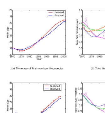
The observed mean age for first marriage frequencies and its variance-corrected values, which correspond toa(t)in equation (8), are depicted in Figure 5(a) for Austria. In the

first half of the 1970s the mean age at first marriage showed a slight drop but starting from 1975 it has been increasing continuously. When correcting additionally for vari-ance distortions, the decrease of the mean age at first marriage would have been more pronounced and hence the corrected mean age was lower than the observed figure till the mid-1980s. This is due to the decrease of variance over the same period of time. With the increase of variance in the mid-1980s, the observed mean age was lower than the corrected one, implying a sharper increase of the variance-corrected mean age over time from 1985 onwards. Since the mid-1990s the increase in the variance-corrected mean age at first marriage has slowed down.

Given the observed changes in tempo, we would expect the Bongaarts-Feeney ad-justed first marriage rate to be lower than the observed TFMR in the first half of the 1970s and to lie above it thereafter. Since the drop in the variance-corrected mean age at first marriage was stronger than in the observed one until the second half of the 1970s, the Kohler-Philipov adjusted TFMR should be even less than the Bongaarts-Feeney adjusted TFMR. Afterwards, the mean age corrected for variance changes increased more strongly until about 1995. Therefore the Kohler-Philipov adjusted TFMR should lie above the Bongaarts-Feeney adjustment between the late 1970s and 1995. As described above, the increase of the variance-corrected mean age at first marriage almost ceased in the second half of the 1990s, and therefore the Kohler-Philipov adjusted TFMR should approach the observed TFMR.

(16)

ad-1970 1975 1980 1985 1990 1995 2000 22 23 24 25 26 27 28 29 Year Mean age corrected observed

(a) Mean age of first marriage frequencies

1970 1975 1980 1985 1990 1995 2000 0.4 0.5 0.6 0.7 0.8 0.9 1 1.1 Year

observed smoothed BF−adjusted KP−adjusted KO−adjusted

(b) Total first marriage rate

1970 1975 1980 1985 1990 1995 2000 25 26 27 28 29 30 31 32 Year Mean age corrected observed

(c) Mean age of first marriage intensities

1970 1975 1980 1985 1990 1995 2000 0.6 0.65 0.7 0.75 0.8 0.85 0.9 0.95 1 Year

Period proportion ever

− married observed smoothed BF−adjusted KO−adjusted

(d) Period proportion ever married

Figure 5: Mean age of female first marriage for Austria, observed and corrected for

(17)

justment factor of the Kohler-Ortega method is derived from the variance-corrected mean age of intensities (cf. Figure 5(c)). The latter slightly decreases until the second half of the 1970s and then strongly increases until the end of the 1980s. From 1990 onwards, the mean age of the intensities, corrected for variance effects, further rises though at a less pronounced rate. The slight decrease followed by a strong increase of the mean age of the intensities causes therefore the down and up observed for the Kohler-Ortega adjusted TFMR in the 1970s and 1980s. Since, the pace of the increase of the variance-corrected mean age of the intensities slows down in the 1990s, the Kohler-Ortega adjusted TFMR decreases again.

Comparing the variance-corrected mean age of the intensities to the observed one, we find that both time series evolve similarly over time, though at different levels, during the first half of the 1970s and during the 1990s. This explains why the Bongaarts-Feeney adjusted PPEM and the Kohler-Ortega adjusted PPEM are almost the same during these periods. Between 1975 and 1990 the variance-corrected mean age of intensities increases more strongly than the observed one, and therefore the Kohler-Ortega adjusted PPEM lies above the Bongaarts-Feeney adjusted PPEM. Finally, since the variance-corrected as well as the observed mean age of the intensities show a slight decrease until about the second half of the 1970s and an increase afterwards, the adjusted PPEM series lie below the observed PPEM until about the second half of the 1970s and above afterwards.

Adjusted for tempo, we see that the period measures show smaller declines in mar-riage than typically reported. The Bongaarts-Feeney adjusted TFMR slightly declined from 1970 to 2000 by about 28 percentage points compared to about slightly more than 40 percentage points by the observed TFMR (cf. Figure 5(b)). The adjustment according to Bongaarts and Feeney (1998a) has a similar effect on the PPEM measure (cf. Fig-ure 5(d)). Instead of dropping by about 30 percentage points, the adjusted series declines just by about 18 per cent.

(18)

Germany

Unfortunately, we were not able to get separate data for former West and East Germany from 1990 onwards. Therefore the results for Germany shown in Figure 6 represent the West German situation in the 1970s and 1980s. From 1990 onwards the results are for West and East Germany combined. However, combining the series for West and East Ger-many from 1990 onwards with only the West German time series prior to 1990 makes the comparison of changes of the tempo and quantum of first marriages over time problem-atic since part of these changes result from compositional rather than behavioural effects. Therefore, we will additionally discuss our results if the data are censored in 1990, i. e. West German data only.

A further problem arises on combining the West and East German time series from the implementation of the adjustment algorithm. From a methodological point of view, the adjustment algorithm should not depend on past values of the time series. However, the smoothing algorithm seems to be sensitive to the initial and terminal value of the corresponding time series. Therefore one should be additionally cautious in interpreting the German results, in particular the values around the unification in 1990.

Other than for Austria, we find a continuously increasing mean age of first marriage frequencies (cf. Figure 6(a)). When correcting for variance distortions, the mean age at first marriage would have been lower until about the early 1980s with only a slight increase. From the early 1980s onwards, the mean age at first marriage corrected for vari-ance effects would have shown a more pronounced increase, which is due to the increase in variance over the same period of time. Summing up, the rate of change of the mean age at first marriage corrected for variance effects over time is greater than the rate of change of the observed mean age at first marriage over the whole investigation period. Hence, the Kohler-Philipov adjusted rates should lie above those adjusted according to Bongaarts and Feeney (1998a).

(19)

1970 1975 1980 1985 1990 1995 2000 0.4 0.5 0.6 0.7 0.8 0.9 1 1.1 Year

1970 1975 1980 1985 1990 1995 2000 0.6 0.65 0.7 0.75 0.8 0.85 0.9 0.95 1 Year

Figure 6: Mean age of female first marriage for Germany, observed and corrected for

(20)

corresponding adjusted TFMR decreases more steeply during this time. Furthermore, the steep rise in the Kohler-Ortega adjusted TFMR during the 1980s corresponds to an equally steep increase in the variance-corrected mean age of the intensities, while the fall of the Kohler-Ortega adjusted TFMR during the 1990s occurs when the mean age of the intensities corrected for variance changes increases at a lesser rate.

Finally, since both the observed and variance-corrected mean age of the intensities increase over the whole investigation period, the adjusted PPEM values lie above the observed values (cf. Figure 6(d)).

Adjusted for tempo, the period measures of first marriage rates show smaller declines in marriage than reported by official statistics over time. Most interestingly, we find that the adjusted total first marriage rates fluctuate heavily, with values ranging between about 0.7 and 0.85 (cf. Figures 6(b)). However, the rise of the adjusted total first marriage rate in the 1990s may be the result of the compositional changes due to the unification of West and East Germany rather than increasing postponement. Therefore, we concentrate only on the changes of tempo and quantum until 1989 in the German case. The decline over time from the beginning of the 1970s until 1989 of the adjusted TFMR is about 17 (Kohler-Philipov) to 18 (Bongaarts-Feeney) percentage points compared to about 29 percentage points of the observed TFMR. Similarly, we find fluctuations in the adjusted PPEM series but with a smaller amplitude and with a clear downward trend of the se-ries (cf. 6(d)). Nevertheless, we focus only on the change over the 1970s and 1980s. The adjusted period proportion ever married declined by about 11 (Kohler-Ortega) or 14 (Bongaarts-Feeney) percentage points from 1971 to 1989 compared to about 17 percent-age points for the observed PPEM series during this period.

Switzerland

For Swiss first marriage rates, we find, similar to the German case, fluctuations in the adjusted series of TFMR and PPEM (cf. Figure 7(b) and Figure 7(d)). However, unlike the German case, these fluctuations are caused by oscillations in the observed TFMR and PPEM series and merely reinforced by the tempo adjustment, since the observed mean ages and the variance-corrected values of their frequencies and intensities show a steady increase over the whole investigation period (cf. Figure 7(a) and Figure 7(c)). The latter also implies that the adjusted series are above the observed TFMR and PPEM series. Since the increase in the mean ages is more pronounced in the 1980s than in the previous and following decades, there are stronger tempo effects in the 1980s (cf. Figure 7(b) and Figure 7(d)).

(21)

1970 1975 1980 1985 1990 1995 2000 0.4 0.5 0.6 0.7 0.8 0.9 1 1.1 Year

1970 1975 1980 1985 1990 1995 2000 0.6 0.65 0.7 0.75 0.8 0.85 0.9 0.95 1 Year

Figure 7: Mean age of female first marriage for Switzerland, observed and corrected

(22)

Bongaarts-Feeney adjusted TFMR lies below the Kohler-Philipov adjusted TFMR during the first two decades and above it thereafter.

Concerning Swiss first marriage intensities, the observed mean ages and their variance-corrected values of Swiss first marriage intensities evolve almost identically over time in the 1970s and 1990s, though at different levels. Hence, the Bongaarts-Feeney adjusted and the Kohler-Ortega adjusted PPEM series are almost the same in that decades. Conse-quently, variance effects in the intensities seem to be absent during the 1970s and 1990s.

3.3 Comparison with Cohort Experience

The most convincing test of the adjustment procedures is perhaps to compare the period measures, adjusted for tempo and variance changes, of first marriage rates with the ex-perience of cohorts, whose marriage proportions are, by definition, unaffected by tempo effects (Goldstein, 2002).

We estimated the completed cohort proportion women who ever married by extrap-olating the observed experience of cohorts using the Coale-McNeil model (Coale and McNeil, 1972) [Note 10]. This model has often been used to forecast cohort marriage rates (Bloom and Bennett, 1990; Goldstein and Kenney, 2001; Liang, 2000). Figure 8(a) shows the cumulative proportions marrying by age of selected cohorts for Austria. The crosses symbolise observed values and the solid line show the fit of the Coale-McNeil model. We see that the predicted proportion marrying by age 50 is falling with each suc-cessive cohort. Though, the estimates for the younger cohorts are based on few observed data points. Moreover, it also appears that the Coale-McNeil model may be underesti-mating late marriage since the model estimates appear to be slightly less than the last observed proportions married for most cohorts.

Figure 8(b) shows the estimated Austrian cohort proportions ever married plotted to-gether with the Austrian period estimates, adjusted for mean and variance changes, that were shown in Figure 5. We have shifted the period measures by their corresponding period mean age of first marriage, where first marriage rates, which were adjusted for mean and variance changes, were shifted by the variance-corrected mean age values. The Kohler-Ortega adjusted measures of first marriage are closer to the cohort forecasts than the other adjustments. However, throughout the total 30 years of investigation, the maximum difference for the five period measures to the cohort proportion ever married amounts to only about 7 percentage points.

(23)

15 20 25 30 35 40 45 50 0

0.1 0.2 0.3 0.4 0.5 0.6 0.7 0.8 0.9

Age

Cumulative proportion of women ever

−married

1955 1960 1965 1970

(a) Cumulative proportions of Austrian women ever married, by cohort

1955 1960 1965 1970

0.5 0.55 0.6 0.65 0.7 0.75 0.8 0.85 0.9 0.95 1

Year

Proportion of women ever

−married

cohort forecast TFMR BF−adjusted TFMR KP−adjusted TFMR KO−adjusted PPEM BF−adjusted PPEM KO−adjusted

(b) Austrian period and cohort measures of first marriage

(24)

15 20 25 30 35 40 45 50 0

0.1 0.2 0.3 0.4 0.5 0.6 0.7 0.8 0.9

Age

−married

1956 1960 1965 1970

(a) Cumulative proportions of German women ever married, by cohort

1955 1960 1965 1970

0.5 0.55 0.6 0.65 0.7 0.75 0.8 0.85 0.9 0.95 1

Year

−married

(b) German period and cohort measures of first marriage

(25)

be too high. The latter may result from the compositional changes due to the unification of East and West Germany rather than from the extrapolation using the Coale-McNeil model. This becomes clear when comparing the estimated cohort proportion ever married to the adjusted period measures. There, we also find increasing values for the translated period series of the late 1960s birth cohorts. However, the Bongaarts-Feeney and the Kohler-Ortega adjusted period measures perform also well in approximating the cohort forecasts for the earlier birth cohorts, which stem from West German data only.

For the Swiss data, the Coale-McNeil extrapolation is given in Figure 10(a). Similar to the Austrian and German cases, we also find a decreasing cohort proportion ever married by age 50 across cohorts. This decline is well approximated by the Kohler-Ortega adjusted values of the translated total female first marriage rates, except of the early 1950s birth cohorts. For the latter the Bongaarts-Feeney adjusted series perform better. However, for all the adjusted period measures the deviation to the cohort forecasts only amounts to about 6 percentage points.

4. Conclusions

In this paper, we have quantified the changes in female first marriage rates for Austria, Germany, and Switzerland in terms of tempo and variance effects by applying methods developed for tempo and variance changes in fertility.

We find a uniform pattern of tempo changes across countries for the different decades. For instance, the 1970s were characterised by a slight increase or even a decrease of mean ages of frequencies or intensities regardless of correcting for variance changes. During the 1980s, postponement of first marriages was severe, since the mean ages steeply increased. Therefore the adjusted values of total first marriages rates as well as the period proportion ever married sharply increase. Finally, the 1990s were characterised by further postponement but at a slower rate than in the previous decade.

(26)

15 20 25 30 35 40 45 50 0

0.1 0.2 0.3 0.4 0.5 0.6 0.7 0.8 0.9

Age

−married

1955 1960 1965 1970

(a) Cumulative proportions of Swiss women ever married, by cohort

1955 1960 1965 1970

0.5 0.55 0.6 0.65 0.7 0.75 0.8 0.85 0.9 0.95 1

Year

−married

(b) Swiss period and cohort measures of first marriage

(27)

Considering variance effects in total first marriage rates, the size of the distortions heavily depends on the method used. This is due to two reasons. First, as stated earlier, the Kohler-Philipov method heavily depends on a technical parameter which can be arbi-trarily chosen (see Note 8). Secondly, using the Kohler-Ortega method, the corresponding intensities are adjusted and then transformed into frequencies. From cohort comparison, we find that Kohler-Ortega adjusted values approximate the cohort forecasts quite well, though with significant deviations for the late 1950s birth cohorts in all three countries. Further investigations including a sensitivity analysis with respect to technical parameters are needed.

To what extent the results depend on the adjustment method used is also apparent by comparing the share of the overall decline in first marriage rates which is attributable to tempo distortions. In particular, the tempo-adjusted decline in total first marriage rates since 1970 is about 36 to 85 per cent of that published in the vital statistics in Austria and Switzerland, which implies a share of 15 to 64 per cent of the reduction in first marriage rates due to tempo distortions [Note 12] However, we also find significant variations of the share of tempo effects across countries, with Switzerland showing the lowest decline due to tempo distortions (20–37 %). The tempo effects in the decline of the total first marriage rate in Austria is significantly higher (33–64 %). However, as evident from Figure 3, Switzerland started in the beginning of the 1970s with a substantially higher mean age at first marriage compared to Austria.

Since there were almost no variance effects in the 1970s and 1990s in the first marriage intensities, the decline in the tempo-adjusted period proportion ever married is nearly independent of the adjustment method used. In particular, the tempo effect amounts to 15 to 34 % of the decline in the period proportion ever married since the 1970s in Austria and Switzerland. Within the countries, we find again Switzerland exhibiting the lowest tempo (15–18 %) and Austria showing much higher values (34 %). Summing up, the proportion of Austrian and Swiss women who will ever marry indeed appears to be declining, but a bit less dramatically than period measures would indicate.

(28)

At the second stage, cohabitations represent predominately a probationary period or a prelude to marriage. This was certainly the case in the late 1970s and in the 1980s. Indeed, 45% of the Austrian marriages in 1989, the bride and the groom were co-residing before marriage (Österreichisches Statistisches Zentralamt, 1993). In the last stages, cohabitation becomes socially acceptable as an alternative to marriage, where cohabitation ends up being almost indistinguishable from marriage (Kiernan, 2001). In fact, Kiernan (2000) finds for data from the European Fertility and Family Survey, which was conducted in the mid to late 1990s, that “cohabitation typically initiates first union and about 30-40 % of the first unions were cohabitations that had converted into a marriage with the same partner.”

Nevertheless, Kiernan (2000) finds for Austrian, German and Swiss FFS data that 52–68 % of the 20–39 year old women with a first partnership were married, which goes along with our finding that the majority of women in the German speaking countries are still marrying once in their lifetimes. However, in Austria the forecast proportion choosing never to marry has risen from 18 per cent for cohorts born in 1955 to an estimated 32 per cent for those born in 1970. Switzerland exhibits somewhat smaller proportions, i.e., 19 per cent of the 1955 birth cohort to an estimated 26 per cent of women born in 1970 in Switzerland (cf. Figures 8(b) and 10(b)).

The tempo findings for Austria are in line with Goldstein’s findings for France. Gold-stein (2002) reports an increase in the proportion women choosing never to marry from about 10 per cent for cohorts born just after World War II to 20 to 30 per cent for the cohorts born in the 1960s. This compares to a level near 50 per cent, as implied by the observed (unadjusted) period measures of marriage.

(29)

5 . Acknowledgements

(30)

Notes

1. We would like to thank Statistik Austria, the Swiss Federal Statistical Office, and the German Statistical Office for supplying the data.

2. Analogous expressions are ‘frequencies’ and ‘incidence rates’.

3. As common in the demographic literature, we restrict our analysis to women between ages 15 to 49 and neglect first marriages of women aged 50 and older.

4. Other expressions commonly used for these rates are ‘occurrence-exposure rates’ and ‘intensities’.

5. One explanation for the very early age at first marriage in 1970, according to Scheller (1985), is the result of a cultural lag. In particular, a change in attitudes towards sexual behaviour took place in the 1960s, implying an increase in pre-marital sexual relation-ships. However, norms about births out of wedlock did not change in the same extent and single mothers as well their illegitimate children were discriminated.

6. Under the framework assumed in Kohler and Ortega (2002), the proof follows straight-forward from the proof of their Result 8 on page 141 by setting the integral limits to the lower and upper age limits of the intensity schedule. Moreover, it can be shown that the equality holds in equation (10).

7. In contrast, Bongaarts and Feeney (1998a) measure the annual rate of change of the mean age at first marriage,(t), according to

^

r(t)=((t+1) (t 1))=2:

8. Kohler and Philipov (2001) recommend to deriveÆ(t)from a regression of the observed

time series of the logarithm of the standard deviation on a polynomial of time (for further details see Kohler and Philipov, 2001). However, we found that the adjusted time series heavily depend on the degree of the polynomial.

9. During our simulations, we found out that the convergence behaviour depends on the right choice of the noise-variance ratio of the smoothing algorithm. Many thanks to Hans-Peter Kohler, who helped us to find the appropriate value of this smoothing parameter.

10. In the Coale-McNeil model, the density of age at first marriage is given by

g(x)=:1946expf :174(x 6:06) exp[ :288(x 6:06)]g;wherex = a a

(31)

(cf. Coale and McNeil, 1972). In particular,ais the age at first marriage,a

0 is the age

at which first marriage may start,scales the speed of entry into first marriage, andis

the proportion of the cohort that eventually marries. The model was estimated with the generalised least square method.

11. However, Sobotka (2003) did not iterate for(t)andÆ(t), which are defined as parameters

from the adjusted frequency or intensity schedule, but computed them from observed values.

(32)

References

Beck-Gernsheim, E. (1998). Was kommt nach der Familie? Einblicke in eine neue

Lebens-form. München: Beck.

Becker, G. S. (1973). A theory of marriage: Part I. Journal of Political Economy 81, 813–846.

Becker, G. S. (1974). A theory of marriage: Part II. Journal of Political Economy,

Supplement 82, S11–S26.

Becker, G. S. (1991). A Treatise on the Family (Enl. ed.). Cambridge: Harvard University Press.

Bloom, D. E. and N. G. Bennett (1990). Modeling American marriage patterns. Journal

of the American Statistical Association 85, 1009–1017.

Bongaarts, J. and G. Feeney (1998a). On the quantum and tempo of fertility. Population

and Development Review 24, 271–291.

Bongaarts, J. and G. Feeney (1998b). On the quantum and tempo of fertility: Reply.

Population and Development Review 26, 560–564.

Bumpass, L. and H.-H. Lu (2000). Trends in cohabitation and implications for children’s family contexts in the United States. Population Studies 54, 29–41.

Calot, G. (1998). Two centuries of Swiss demographic history. Neuchâtel and Paris: Swiss Federal Statistical Office and Observatoire démographique européen.

Cherlin, A. J. (2000). Toward a new home socioeconomics of union formation. In L. J. Waite (Ed.), The Ties that Bind: Perspectives on Marriage and Cohabitation, Chap-ter 7, pp. 126–144. New York: Aldine de GruyChap-ter.

Coale, A. J. and D. R. McNeil (1972). The distribution by age of the frequency of first marriage in a female cohort. Journal of the American Statistical Association 67(340), 743–749.

Diekmann, A. (1987). Determinanten des Heiratsalters und des Scheidungsrisikos. Un-veröffentlichte Habilitationsschrift, Universität München, Institut für Soziologie.

Engelhardt, H. (2002). Zur Dynamik von Ehescheidungen: Theoretische und empirische

(33)

Ermisch, J. and M. Francesconi (2000). Cohabitation in Great Britain: not for long, but here to stay. Journal of the Royal Statistical Society, Series A 163, 153–171.

Gisser, R., L. Wilk, M. Beham, and M. Bacher (1990). Familiale Wirklichkeit aus de-mographischer und soziologischer Sicht. In R. Gisser, L. Reiter, H. Schattovits, and L. Wilk (Eds.), Lebenswelt Familie. Wien: Institut für Ehe und Familie.

Goldstein, J. R. (2002). The tempo and quantum of first marriage. Draft.

Goldstein, J. R. and C. T. Kenney (2001). Marriage delayed or marriage foregone? New cohort forecasts of first marriage for U.S. women. American Sociological Review 66, 506–519.

Goode, W. J. (1982). The Family. Englewood Cliffs, NJ: Prentice Hall.

Heckman, J. J., V. J. Hotz, and J. R. Walker (1985). New evidence on the timing and spacing of births. American Economic Review 75, 179–184.

Heilig, G. (1985). Die Heiratsneigung lediger Frauen in der Bundesrepublik Deutschland: 1950–1984. Zeitschrift für Bevölkerungswissenschaft 11(4), 519–547.

Kiernan, K. (1999). Cohabitation in Western Europe. Population Trends 96, 33–40.

Kiernan, K. (2000). European perspectives on union formation. In L. J. Waite (Ed.),

The Ties that Bind: Perspectives on Marriage and Cohabitation, pp. 40–58. New York:

Aldine de Gruyter.

Kiernan, K. (2001). The rise of cohabitation and childbearing outside marriage in Western Europe. International Journal of Law, Policy and the Family 15, 1–25.

Kim, Y. J. and R. Schoen (2000). On the quantum and tempo of fertility: Limits to the Bongaarts-Feeney adjustment. Population and Development Review 26, 554–559.

Kohler, H.-P. and J. A. Ortega (2002). Tempo-adjusted period parity progression measures, fertility postponement and completed cohort fertility. Demographic

Re-search 6(6), 91–144.

Kohler, H.-P. and D. Philipov (2001). Variance effects in the Bongaarts-Feeney formula.

Demography 38, 1–16.

Lesthaeghe, R. (1995). The second demographic transition in Western countries: An interpretation. In K. O. Mason and A.-M. Jensen (Eds.), Gender and Family Change in

(34)

Liang, Z. (2000). The Coale-McNeil Model: Theory, Generalisation and Application. Amsterdam: Thela Thesis.

Lundberg, S. and R. A. Pollak (1996). Bargaining and distribution in marriage. Journal

of Economic Perspectives 10(4), 139–158.

Lutz, W., B. O’Neill, and S. Scherbov (2003). Europe’s population at a turning point.

Science 299, 1991–1992.

Manting, D. (1996). The changing meaning of cohabitation and marriage. European

Sociological Review 12, 53–65.

McLanahan, S. and G. Sandefur (1984). Growing Up with a Single Parent: What Hurts,

What Helps. Cambridge: Harvard University Press.

Murphy, M. (2000). The evolution of cohabitation in Britain, 1960-95. Population

Stud-ies 54, 43–56.

Ng, C. N. and P. C. Young (1990). Recursive estimation and forecasting of non-stationary economic times series. Journal of Forecasting 9(2), 173–204.

Oppenheimer, V. K. (1988, November). A theory of marriage timing. American Journal

of Sociology 94(3), 563–591.

Oppenheimer, V. K. (2000). The continuing importance of men’s economic position in marriage formation. In L. J. Waite (Ed.), The Ties that Bind: Perspectives on Marriage

and Cohabitation, Chapter 14, pp. 283–301. New York: Aldine de Gruyter.

Oppenheimer, V. K. and A. Lewin (1999). Career development and marriage formation in a period of rising inequality: Who is at risk? What are their prospects? In A. Booth, A. C. Crouter, and M. J. Shanahan (Eds.), Transitions to Adulthood in A Changing

Economy: No Work, No Family, No Future?, Chapter 13, pp. 189–225. Westport, CT:

Greenwood Press.

Österreichisches Statistisches Zentralamt (Ed.) (1988). Demographisches Jahrbuch 1986, Wien. Österreichisches Statistisches Zentralamt.

Österreichisches Statistisches Zentralamt (Ed.) (1993). Demographisches Jahrbuch 1992, Wien. Österreichisches Statistisches Zentralamt.

Péron, Y. (1991). Les indices du moment de la nuptialité des célibataires.

Popula-tion 46(6), 1429–1440.

(35)

Prioux, F. (1992). Les accidents de la nuptialité autrichienne. Population 47, 353–388.

Scheller, G. (1985). Erklärungsversuche des Wandels im Heirats– und Familiengrün-dungsalter seit 1950. Zeitschrift für Bevölkerungswissenschaft 11(4), 549–576.

Sobotka, T. (2003). Tempo-quantum and period-cohort interplay in fertility changes in Europe: Evidence from Czech Republic, Italy, the Netherlands and Sweden.

Demo-graphic Research 8(6), 151–214.

Statistik Austria (Ed.) (2001). Demographisches Jahrbuch 2000, Wien. Statistik Austria.

Statistik Austria (Ed.) (2003). Demographisches Jahrbuch 2001–2002, Wien. Statistik Austria.

The MathWorks, Inc. (2002). Matlab 6.5.

Toulemon, L. (1997). Cohabitation is here to stay. Population: An English Selection 9, 11–56.

van Imhoff, E. and N. Keilman (2000). On the quantum and tempo of fertility: Comment.

Population and Development Review 26, 549–553.

Waite, L. (1995). Does marriage matter? Demography 32, 483–507.

Yi, Z. and K. C. Land (2001). A sensitivity analysis of the Bongaarts-Feeney method for adjusting bias in observed period total fertility rates. Demography 38, 17–28.

(36)