in the population sciences published by the Max Planck Institute for Demographic Research Konrad-Zuse Str. 1, D-18057 Rostock·GERMANY www.demographic-research.org
DEMOGRAPHIC RESEARCH
VOLUME 15, ARTICLE 16, PAGES 461-484
PUBLISHED 28 NOVEMBER 2006
http://www.demographic-research.org/Volumes/Vol15/16/ DOI: 10.4054/DemRes.2006.15.16
Reflexion
Anticipatory analysis and its alternatives
in life-course research.
Part 1: The role of education
in the study of first childbearing
Jan M. Hoem
Michaela Kreyenfeld
c
°2006 Hoem & Kreyenfeld
1 Introduction 462
2 Education and fertility 464
2.1 Anticipatory indicators of the impact of educational attainment on fertility 464
2.1.1 Cross-sectional fertility indicators 464
2.1.2 Reflections 465
2.1.3 Survival curves by final level of education 467
2.2 Allowing education to vary over time 469
2.2.1 An event-history model incorporating the combination of current educa-tional level and enrolment in education as a time-varying covariate 469
2.2.2 Survival curves by current educational attainment 471
2.3 Accounting for the interrelation between childbearing and educational
at-tainment 474
3 Conclusion 478
4 Acknowledgement 480
References 481
Anticipatory analysis and its alternatives in life-course research.
Part 1: The role of education in the study of first childbearing
Jan M. Hoem1
Michaela Kreyenfeld2
Abstract
Procedures that seek to explain current behavior by future outcomes (anticipatory analy-sis) constitute a widespread but problematic approach in life-course analysis because they disturb the role of time and the temporal order of events. Nevertheless the practice is often used, not least because it easily produces useful summary measures like the median age at first childbearing and the per cent permanently childless in various educational groups, defined by ultimate attainment. We use an empirical example to demonstrate the issues involved and to propose an alternative “non-anticipatory” research strategy that makes use of the incomplete data most commonly collected. A weakness of the latter method is that to make things work it builds on assumptions that may be unrealistic, and still it does not equally easily provide summary measures. There is no satisfactory alternative to better data collection.
1.
Introduction
Time and the temporal order of events play a decisive role for our understanding of be-havioral processes that evolve over time in an individual’s life. The topic of this paper is anticipatory analysis, which is any approach where one attempts to explain past or current behavior by future outcomes, in other words by conditioning on the future. It is important to understand the function and outcome of such a practice, for it remains quite popular. Here are a couple of typical examples that have appeared recently in the best of demographic journals:
(i) In a paper in Demography concerned with first-birth rates for women above age 30, Martin (2000) analyzed complete fertility histories from the U.S. Current Population Survey using educational attainment measured at the date of interview as an explanatory variable. The analysis most often3 is anticipatory because the educational outcome is known only at the end of the periods for which fertility behavior is recorded. The practice is ubiquitous and we refrain from a literature review.
(ii) In a paper in the Journal of Marriage and the Family, Corijn, Liefbroer and Gierveld (1996) also study entry into motherhood. One of their regressors is religious affiliation measured at the date of interview. When religious affiliation is not fixed over the life-course, their analysis is anticipatory. De Wit and Ravanera (1998) followed the same practice in a similar study, as did Hoem and Hoem (1989).
A considerable literature warns against the use of an anticipatory approach (see, e.g., Hoem 1996; Kravdal 2004), but researchers vary in their attitudes. An advantage of anticipatory analysis is that it sometimes easily provides descriptive summary measures of demographic behavior (like the median ages at first birth and the percentage ultimately childless by ultimate educational attainment, as in Figure 1 below), while this can be much harder with a non-anticipatory approach. Such summary measures can be useful to layman and professional alike, because they encapsulate important consequences of the transition rates that are so popular among life-history analysts. We therefore address the following general questions: Must anticipatory analysis produce biased results? Is it not rather a research tool that can be used to discover patterns of social processes, patterns that might be hard to reveal otherwise? In particular, can conditioning on the future be an acceptable research strategy when educational histories are not available but educational attainment at the time of interview is? Is an anticipatory approach misleading when it is used for causal inference but still acceptable for descriptive purposes? Or is the outcome of some anticipatory analysis deceptively and misleadingly simple, and are such procedures a total malpractice that violates basic principles of statistical methodology,
3There may be an exception in the rare cases where essentially all women really complete all education
perhaps by regularly producing biased results? By extension, we ask which strategies are available to avoid anticipatory analysis.
The authors of these reflections have found a need to discuss such issues extensively with each other.4The purpose of the present text is to share our considerations with others
and to display various possible procedures of analysis. For those who like to know where the road leads to, let us note at the outset that we have found the easy descriptions pro-duced by an anticipatory analysis enticing but potentially deceptive, in that they may give a seriously biased and overly simplified impression of the patterns of real behavior. We offer an alternative procedure that is not anticipatory and not subject to the same flaws. It is an elementary extension of ordinary life-table theory. It exploits a particularly sim-ple representation of educational-and-childbearing histories where all that is known is the educational level attained at the time of interview and the age at which it was attained, from which we impute a rudimentary educational history. This type of data occurs often in practice, and the procedure we present works most straightforwardly where the edu-cational system is quite rigid. It can be generalized to situations where more complete histories have been collected and where the educational system is more flexible, but that is not part of our account here.
Of course the procedure we propose builds on a simplification of reality too, but at least it has the advantage of representing education and childbearing explicitly as two dynamic processes. We trust that the simplification does not in itself produce distortions that lead readers to a new set of misunderstandings. We illuminate these considerations by working through an empirical example based on real data in the sections that follow, and we do the same for the connection between marriage formation and childbearing in our companion paper (Hoem and Kreyenfeld 2006). We believe that the examples have some independent interest in their own right. Unfortunately, the procedure we propose does not provide anything like a median age at first childbearing or a percentage ultimately childless by educational attainment, except by conditioning on the ultimate level of the latter, thus returning to the anticipatority strategy we set out to eliminate in the first place. We want to underline that we do not offer the non-anticipatory procedure described in this paper as a general alternative to better (i.e., more complete) data collection. Quite on the contrary, by displaying the simplifying assumptions needed to make things work here, we aim to highlight the hopelessness of basing sensible analysis in general on the overly sparse information collected as a standard procedure. There is no way around the fact that good data are better than (even good) methodology whose function it is to patch up the weaknesses of incomplete data. Hopefully our procedure may work in special cases, like possibly the data set we apply it to. In future work we hope to demonstrate the gain
4After submission we got involved in further enlightening discussions with the journal’s reviewers, to whom
attained from using more complete data. For the moment we concentrate on blowing the whistle.
2.
Education and fertility
2.1 Anticipatory indicators of the impact of educational attainment on fertility
2.1.1 Cross-sectional fertility indicators
The connection between education and family dynamics has been discussed intensively in demographic, economic, and sociological work. (See, e.g., Hoem 1986; De Wit and Ravanera 1998; Blossfeld and Huinink 1991; Liefbroer and Corijn 1999; Santow and Bracher 2001.) The standard reasoning is that more highly educated women spend longer periods of their lives in education; when they enter the labor market, they earn higher wages, are more work-oriented, and enter more challenging employment careers. All of these factors are thought to work towards postponing family formation and increase childlessness. Here are some immediate questions: How old are university graduates when they have their first child? How many of them remain childless throughout their lives? And how is their behavior in comparison to other women?
To answer such questions it would be useful to have easily accessible summary indi-cators. Some obvious examples are the mean or median age at first birth and the fraction permanently childless among the women in each educational subgroup. Such indicators are used frequently in demographic research (see, e.g., Rindfuss, Morgan and Offutt 1996; Björklund 2006). They are also of major public interest. A high percentage childless (for instance) in any group may suggests a strong incompatibility between work and family life in that group. In the recent public debate in Germany, the published finding that uni-versity graduates have particularly high levels of childlessness has found strong resonance among politicians and the public (Bernd 2005). Since such indicators are easily picked up by a wider audience, they are possibly better suited to promote political action than complex indicators derived from more sophisticated analytical strategies are.
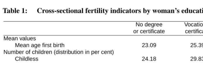
In Table 1, we display some cross-sectional fertility indicators. The data for this and all subsequent analysis come from the German Family and Fertility Survey (FFS), con-ducted in 1992. We have selected West German women of ages 30-39 at the time of the interview and have grouped them into three categories according to the highest ed-ucational level they have attained by the time of the interview, namely women with (i) a university degree, (ii) a vocational-training certificate, and (iii) none of these attain-ments.5 The table shows a strong association between recorded educational attainment
5What we have called university degree includes ‘Fachhochschulabschluss’ and ‘Hochschulabschluss’.
and fertility. According to the table, university graduates were the older at first birth, they were much more likely than others to remain childless, and on average they gave birth to a smaller total number of children than other women.
Table 1: Cross-sectional fertility indicators by woman’s educational level.
No degree Vocational University
or certificate certificate degree
Mean values
Mean age first birth 23.09 25.39 28.17
Number of children (distribution in per cent)
Childless 24.18 29.83 48.28
One child 19.28 28.23 14.48
Two children 34.64 33.83 24.83
Three and more children 21.90 8.11 12.41
Total 100.0 100.0 100.0
Mean total number of children 1.54 1.20 1.01
Source: German FFS 1992 (our own estimates).
2.1.2 Reflections
According to Table 1, childlessness at ages 30-39 was radically more common among university graduates than among other educational groups. A straightforward and com-mon explanation is that highly educated women are the more career-oriented, and that they remain childless to a large extent because work and family life are not easily com-patible in Germany. This is probably true, but we have a number of reservations to simply basing the argument for it on statistics like those in Table 1 and to the quantifications that the table contains.
First, the interpretation just mentioned is plainly wrong to the extent that causality works in the opposite direction. Suppose that a woman must discontinue her university studies because she has a child. For her it is not (lack of) career orientation that makes her have fewer children; quite on the contrary her childbearing limits her educational choices. If this pattern is common, the table would only provide limited insight into the causal relationship between education and first birth. For another example, suppose a woman completes some vocational training at age 20 and has a child at 21. At age 28,
she goes back to take more education, and she receives a university degree at age 32. Her fertility choice was probably made before she even contemplated going to the university. Nevertheless she would be classified as a university graduate in Table 1. This amounts to a time-sequence reversal, which is a dangerous practice in itself. These examples show that conclusions about decision processes cannot be based on statistics like those in Table 1.
A fertility indicator computed by final educational level in some sense assumes that education is a fixed trait of the individual. How sensible this is, depends on the struc-ture and flexibility of the educational system. If education is completed regularly before childbearing begins, a causal interpretation of fertility by final level of education may be meaningful, because then it does not matter when educational attainment is measured. The more that people pursue extended or multiple educational careers and the more they re-train at later ages, the less meaningful it is to use education as a fixed characteristics of an individual, because such re-orientation takes time and is likely to stretch into the childbearing period. The only alternative apparent to us that makes the anticipatory pro-cedure meaningful is to see ultimate educational attainment as revealing a lifetime plan which guides the individual’s behavior until completion and which therefore is a fixed characteristic. We are skeptical of such a teleological interpretation.
Second, a related problem arises from the fact that some women do not have a de-gree yet, but are in education on the date of interview in order to complete their studies. We coded them as not having any degree or certificate. Even though this classification is formally correct, this does not seem to be a particularly sensible solution. Those still enrolled in education are most likely undergoing university education. Prospective uni-versity graduates (who just have not finished by the time of the interview) will behave differently from women who have completed their education at a lower level or have dropped out of education without having earned a degree or certificate. One could omit from the analysis women who are in education, but this solution has its own problems. It biases the results because women who are under education at interview surely include those who postpone fertility longer than others. Alternatively, one could classify them as university graduates, but this procedure would not account for university drop-outs.
aged 45-60 at interview, a retrospective fertility study mainly reflects childbearing behav-ior some twenty to thirty years ago on average. More up-to-date fertility indicators would certainly be preferable for those interested in current trends.
Survival analysis has been devised to account for censoring and to allow us to analyze the fertility of cohorts who are still in their reproductive years. A summary statistic like the median age at first birth can be derived from survival curves. We now turn to this possibility.
2.1.3 Survival curves by final level of education
Figure 1 shows survival curves for time to first birth, by level of education attained at interview for our 30-to-39-year-olds. These survival curves explicitly take censoring of the main event (childbearing) into account, but they too treat education as a fixed per-sonal trait. In principle, our respondents came under the risk of childbearing at age 15. Everything that happened before this age is fixed for the first-birth process. (For example, the woman’s own place and year of birth trivially are fixed factors.) We recapitulate that this is not so for educational attainment; this factor varies over the life-course. At age 15, none of the respondents has a vocational certificate or a university degree yet. On average, a vocational certificate is earned at age 19 in this data set, a university degree at age 28. When respondents are classified throughout their life histories (as far as we have observed them) according to educational attainment at interview, their educational level is essentially wrongly coded during life segments before they attain that “final” level. For instance, the first-birth survival curve for university graduates provides estimates for the fraction childless at ages 15 to 19, but at such ages no university degree has been earned. We derive the following Table 2 from the diagram. A comparison with corresponding entries in Table 1 shows considerable adjustment of the figures for university graduates but only smaller changes for those with a lower educational attainment. We get these changes because Table 2 catches the women at an age on average five years later than in Table 1. (Note that for those with a university degree the median age in Table 2 is more than five years higher than the corresponding mean in Table 1.)
Figure 1: Kaplan-Meier survival curves for the arrival of the first child, by final level of education
Note: Computations based on data for West German women aged 30 to 39 at interview. Source: German FFS 1992 (our own estimates)
Table 2: Median age at first birth and per cent childless at age 40, by educational attainment at interview, based on Figure 1.
No degree Vocational University
or certificate certificate degree
Median age at first birth6 24.00 27.67 33.67
Childlessness at age 40, in per cent 21.50 26.03 41.21
Source: German Family and Fertility Survey 1992 (our own estimates).
time-varying covariate is safer, particularly in that it minimizes the risk of estimation bias. To get a closer look at these issues, we now turn to the latter option.
2.2 Allowing education to vary over time
2.2.1 An event-history model incorporating the combination of current educational level and enrolment in education as a time-varying covariate
A major advantage of an event-history approach is that it makes it possible to consider education as a time-varying determinant of the behavior in focus, in our case first child-bearing (see e.g., Hoem 1986; De Wit and Ravanera 1998; Blossfeld and Huinink 1991; Liefbroer and Corijn 1999; Santow and Bracher 2001). An essential requirement is that the data contain information about the respondent’s educational attainment and any cur-rent educational enrolment for each month during the period of observation. Unfortu-nately, such detail is not always available, and the German FFS is a case in point. In that survey, respondents were “only” asked to report the highest educational level they had attained at the time of interview and the month and year in which they completed that education. They could choose between nine different educational levels, which we have regrouped into the three categories mentioned above (university degree completed, voca-tional certificate earned, and none of these). We have also constructed a (time-varying) binary variable that we hope will indicate periods in and out of education reasonably faith-fully. We coded the respondents as being in education all the time before they attained the level reported in the interview. After the date of completion reported, we coded them as out of education. For respondents who had never attained a university-level degree or a vocational certificate, no real completion date was reported, and we have imputed a drop-out-date from education for each member of this rather heterogeneous group7 and have
coded her as in education until the drop-out date. Respondents who reported a vocational certificate as their highest educational attainment, were coded as being “in education” until the completion of the certificate. Respondents who reported a university-level edu-cation, were coded as being “in education” until completion of the university degree. It is obvious that this practice gives a simplified representation of reality. It does not account for more complex and diverse educational histories. Cases are not adequately considered where people receive multiple degrees and where they resume education after periods of employment. There may also be other, less obvious types of miscoding. However, the
7To impute the drop-out-date, we proceed as follows. For most cases, we know the date when the woman
way education was surveyed in the German FFS, we do not have much choice.8 At least
our procedure has the merit of simplicity. It should also be sufficiently accurate for our methodological purpose.
With educational histories imputed as just described, we have fitted an event-history model to the data. Our process time is the age of the woman, used in the interval from age 15 to age 39, which we have partitioned by cut-points at ages 20, 25, and 30. The baseline hazard is essentially modeled as a function which is piecewise constant over the resulting four intervals.9Educational level and educational activity were entered together
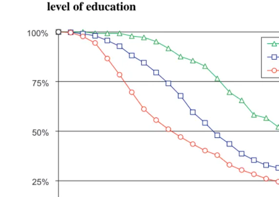
as a combination factor, in that we combined educational activity and educational level into a single time-varying covariate with the values indicated in the head of Table 3 below. Let us call it current educational attainment to underline that education is accounted for in a dynamic way. We use a continuous-time approach, but we cannot use a straightfor-ward multiplicative-hazard model for the effects of these two covariates (age and current educational attainment), and we have included them in interaction. Since no respondent can reach the highest educational level at a very young age, some combinations of age and current educational attainment are impossible in practice, as is indicated by the minus signs in one corner of Table 3. Figure 2 contains a plot of the absolute risks against age for the four columns in that table. It shows how the first-birth risks vary by age and ed-ucational attainment. Note how there is not monotonic dependence between eded-ucational attainment and childbearing risk across all ages.
Table 3: First-birth risk by age and current educational attainment, per 1000 woman-months.
Enrolled in Not enrolled, Not enrolled, Not enrolled,
education no degree or certificate vocational certificate university degree
k 0 1 2 3
15−19 1.02 6.64 3.67 –
20−24 1.38 9.50 5.77 8.74
25−29 1.96 7.20 9.57 6.24
30−39 2.50 4.34 4.60 5.91
Notes: The sample comprises West German women aged 30 to 39 at the time of interview. Source: German Family and Fertility Survey 1992 (our own estimates).
8In fact, our quandary can serve as a warning to data collectors who believe that they can get away with
the bare-bones information about educational histories used in the German FFS and many other similar surveys.
Figure 2: First-birth risk by age and current educational level, per 1000 woman-months
Notes: Data from Table 3
Source: German Family and Fertility Survey 1992 (our own estimates).
2.2.2 Survival curves by current educational attainment
In some sense the results of Section 2.2.1 represents the answer to the substantive ques-tions we have asked. A wider audience may find the consequences of hazard curves such as those in Figure 2 rather inaccessible, however, and the professional would also find some summary measures useful as indicators of what curves like these mean for the age at childbearing and the per cent permanently childless. It may be easier to interpret what the curves mean if we convert them to a format similar to the survival curves in Figure 1. One possibility is then to provide survival curves by current educational level. To do so, we proceed as follows.
Fork= 0,1,2,3, letϕk(x)be the first-birth hazard for a respondent whose current educational attainment at (exact) agexisk, and fork = 1,2,3let the corresponding single-intensity survival function10be
10We remind the reader that such functions are computed under the anti-factual assumption that the given
lk(x) = exp
−
x
15ϕk(s)ds
for x≥15.
(The value ofk is given in the heading of each column in Table 3.) We can then use estimatesϕˆk(x)such as those in Table 3 to produce corresponding estimates for the survival functions. For illustration, let us calculate the points of the survival function for the ages 20, 25, 30 and 40 for women with a vocational certificate (k= 2). Since there are sixty months in each five-year interval and since the items in the table are given per 1000 person-months, we get
ˆ
l2(20) = exp
−601000∗3.67
= 0.80;
ˆ
l2(25) = ˆl2(15)∗exp
−601000∗5.77
= 0.57;
ˆ
l2(30) = ˆl2(25)∗exp
−601000∗9.57
= 0.32; and
ˆ
l2(40) = ˆl2(30)∗exp
−1201000∗4.60
= 0.18.
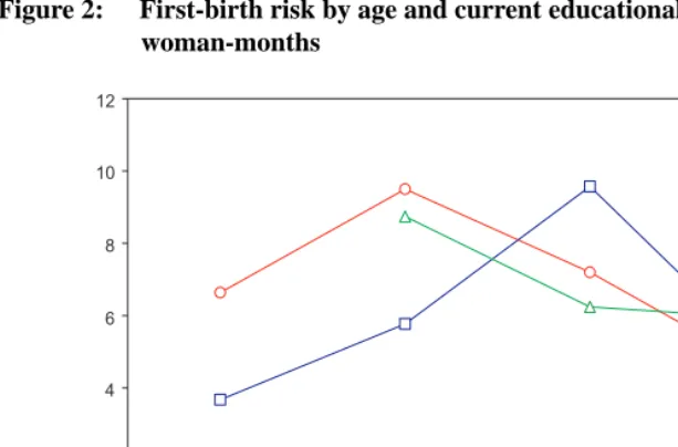
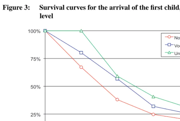
After similar computations for the variousˆlk(x)fork= 1andk = 3, we can draw survival curves like those in Figure 3,11 from which we derive the mean ages at first
birth and the percentages childless in Table 4 corresponding to the values in Table 2. A comparison between Tables 2 and 4 shows that the use of single-intensity functions gives a picture of the role of education that is completely different from what we got by conditioning on educational attainment at interview. In particular, by this account the behavior of women with a university degree is far less radically different from other women that what the anticipatory analysis indicated. According to this analysis, “only” twenty per cent of university-educated women were childless at age 40 (instead of 41% as estimated by the anticipatory analysis and even 48% as estimated in the descriptive analysis of Table 1). Their median age at first birth is just over 27, which is more than six years lower than what the anticipatory analysis gave.
11We could have computedˆl
Figure 3: Survival curves for the arrival of the first child, by currenteducational level
0% 25% 50% 75% 100%
15 20 25 30 35 40
No degree Vocational certificate University degree
Age of woman (years)
Table 4: Median age at first birth and per cent childless at age 40, by current educational level, based on Figure 3.
No degree Vocational certificate University degree
Median age at first birth 22.94 26.36 27.49
Childless at age 40, in per cent 14.65 18.39 20.03
2.3 Accounting for the interrelation between childbearing and educational attain-ment
It would be neat if we could stop here and say that our analysis has proved irrevocably that the anticipatory analysis gives terribly biased results and that the truth is quite dif-ferent from what the anticipatory analysis shows. Unfortunately, things are not quite so simple. Our results in Section 2.2 do not immediately represent a “truth” that anticipatory analysis can be compared with. It is important to note that the single-intensity survival functionslk(x)are constructs that must be interpreted with considerable care themselves, for they do not take into account that educational attainment may change over the period of childbearing. Both educational progress and first childbearing are dynamic processes, and we need to take them both into consideration at the same time. This can be done as follows.
The first-birth intensitiesϕk(x)(k= 0,1,2,3)are picked from a model that incorpo-rates both processes. A simple representation of this model is given in Figure 4, where the boxes represent life-course statuses that individuals can move between and the arrows reflect direct transitions that individuals can make. The functions associated with the ar-rows are corresponding transition intensities (or hazards). The intensitiesγ1(x),γ2(x), andγ3(x)are age-specific rates at which childless individuals change educational status for each agex. Thusγ1(x)is the rate at which they leave the educational system with-out formally completing either a vocational certificate or a university-level degree, while
γ2(x)andγ3(x)are the rates at which they leave the educational system with a vocational certificate or a complete university degree, respectively. Because of the character of the FFS data at our disposal, we have needed to simplify central features of the German edu-cational system, and the peculiarities of our representation are reflected as follows:
(1) Individuals remain in the state marked START (“no child, enrolled, ed = 0”) as long as they are enrolled in education and until they enter motherhood or else complete a certificate or degree.
(2) Once an individual has left the educational system, there is no return.
(3) If an individual leaves the educational system without a vocational certificate or a university degree before entering motherhood, she moves to educational level 1 and remains there forever after.
(4) If they do not drop out, enrolled individuals can complete their education by ac-quiring a vocational certificate (which means that they go to educational level 2) or by completing university studies (educational level 3).
Figure 4: Status-and-transitions diagram for education and first childbearing.
no child, enrolled, ed = 0
no child, not enrolled,
ed = 1
no child, not enrolled,
ed = 2
no child, not enrolled,
ed = 3
with child,
ed = 0 with child,ed = 1 with child,ed = 2 with child,ed = 3
Start
k=1
k=2
k=3
j0(x) j1(x) j2(x) j3(x)
g3(x)
g2(x)
g1(x)
Note that our specification does not allow for education that is continued after first birth. It “only” accounts for the impact of education on first childbearing.
Note that this specification makesγ1(x),γ2(x),γ3(x), andϕ0(x)the intensities (or hazards) of competing risks of transition out of the state marked START in Figure 4, whileϕ1(x),ϕ2(x), andϕ3(x)are intensities of the only possible transition out of their respective states.12 If we letk= 0represent the “educational attainment” corresponding to being enrolled in education and having no child (i.e., location in state START), then the survival function corresponding to this situation would be
l0(x) = exp
x
15[ϕ0(s) + 3
j=1
γj(s)]ds
for x≥15.
This would be the probability of not leaving the status “No child, enrolled, ed=0” (the state marked START) before agex.
12We could have let the three latter transition intensities depend on time since educational attainment (i.e.,
Fork= 1,2,3,lk(x+t)/lk(x) = exp
−0tϕk(x+s)ds
is the probability that an individual will remain in the status marked “No child, not enrolled, ed=k” until agex+t, given that she has reached that status by agex. Both of these exponential formulas are derived in the same manner as when we compute a normal life-table survival probability by forming
tpx=lx+t/lx= exp
−
t
0 µx+sds
when the hazard rate isµx.
The probability of having become a mother and also having reached ed=k (i.e., one of the lowermost states in Figure 4) by agexis
π0(x) =
x
15l0(s)ϕ0(s)ds
fork= 0,
πk(x) =
x
15l0(s)γk(s)
1−lk(x)
lk(s)
ds for k= 1,2,3.
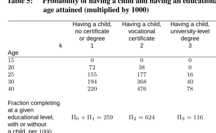
For some empirical values, see Table 5. (The columns of Table 5 are estimates of
π0(x)+π1(x), π2(x), π3(x),and their sum, respectively, for the various agesxindicated.) Table 5 contains a considerable amount of information about the moves individuals have made in the two dimensions we operate in (educational attainment and first child-bearing). Among other features we see that about one-quarter of the respondents in our cohort ended up without a vocational certificate or university-level degree by age 40, that some 15 per cent ended up childless and with a vocational certificate, while about one-fourth as many ended up at childless but with a university-level degree at age 40. The latter is about the same fraction that ended up childless and without any education at those two higher levels.
We have not been able to devise a measure similar to the median ages at first birth by educational attainment in Tables 2 and 4, except by appealing once more to an anticipatory procedure. We do the latter as follows.
LetΠ0=π0(40) =
40
15 l0(s)ϕ0(s)ds
and letΠk =
40
15 l0(s)γk(s)ds
fork= 1,2,3.
Table 5: Probability of having a child and having an educational attainment, by age attained (multiplied by 1000)
Having a child, Having a child, Having a child, Having a child, no certificate vocational university-level all educational
or degree certificate degree attainments together
k 1 2 3
Age
15 0 0 0 0
20 72 38 0 111
25 155 177 16 348
30 194 368 40 601
40 220 476 78 774
Fraction completing at a given
educational level, Π0+ Π1= 259 Π2= 624 Π3= 116 Πk= 1000
with or without a child, per1000
Fraction ending childless and
at a given level 38 148 38 225
of educational attainment, per1000
Notes: The sample comprises West German women aged 30 to 39 at the time of interview. Source: German Family and Fertility Survey 1992 (our own estimates).
by age 40, andΠ0+ Π1is the corresponding probability of remaining at a lower educa-tional level. The condieduca-tional probability that a woman became a mother before age x, given that she reached educational levelkby age 40, is therefore[π0(40) +π1(40)/Π0+
Π1]fork= 1, and it is[πk(40)/Πk]fork= 2or3. All of these conditional probabilities can be estimated from our data and plotted in the form of survival curves13as in Figure 5, from which we can derive Table 6.
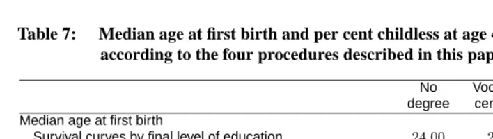
In the reflections above, we have described four different ways of producing median age at first birth and per cent permanently childless by educational attainment. To provide a summary of our findings, we list the main traits of our previous tables (Table 7). We see that the mean ages at childbirth computed according to the ideas of the present section are pretty close to (but not identical with) those computed by organizing the data according to educational attainment observed at interview. However, our approach provides vastly
13The curves plotted fork = 2and3are for the functions1−π
Figure 5: Survival curves for the arrival of the first child, accounting for the interrelation between childbearing and educational attainment.
0% 25% 50% 75% 100%
15 20 25 30 35 40
Age of woman (years)
No degree Vocational certificate University degree
different levels of final childlessness by educational level. The main advantage of the new measures is that they better reflect that education is a time-varying factor in the first birth process. Crudely plotting survival curves by ultimate educational attainment, as in Figure 1, misses out on the interaction between the two individual-level processes involved.
3.
Conclusion
Table 6: Median age at first birth and per cent childless at age 40, accounting for the time-varying nature of education in the first birth process, based on Figure 5.
No degree Vocational certificate University degree
Median age at first birth 23.47 28.54 32.42
Childlessness at age 40 (per cent) 14.74 23.79 33.10
Source: German Family and Fertility Survey 1992 (our own estimates).
Table 7: Median age at first birth and per cent childless at age 40, computed according to the four procedures described in this paper.
No Vocational University
degree certificate degree
Median age at first birth
Survival curves by final level of education 24.00 27.67 33.67
Survival curves by current educational attainment 22.94 26.36 27.49
Accounting for interrelation between education and fertility 23.47 28.54 32.42 Childlessness at age 40 (per cent)
Survival curves by final level of education 21.50 26.03 41.21
Survival curves by current educational attainment 14.65 18.39 20.03
Accounting for interrelation between education and fertility 14.74 23.79 33.10
Source: German Family and Fertility Survey 1992 (our own estimates).
have multiple educational careers and can re-train at later ages, the more problematic is treating education as a fixed characteristic.
4.
Acknowledgement
References
Bernd, Ulrich (2005): “Warum habt ihr Angst vor mir? Akademiker bekommen immer weniger Kinder. Sie sind keine Egoisten. Ihnen fehlt auch nicht das Geld. Sie haben blo"s keinen Mut.” Die Zeit 08/2005.
Björklund, Anders (2006): “Does family policy affect fertility?” Journal of Population Economics, 19: 3-24.
Blossfeld, Hans-Peter and Huinink, Johannes (1991): “Human capital investment or norms of role transition? How women’s schooling and career affect the process of family formation”, American Journal of Sociology 97(1): 143-168.
De Wit, Margaret L. and Ravanera, Zenaida R. (1998): “The changing impact of women’s educational attainment on the timing of births in Canada.” Canadian Studies in Pop-ulation 25(1): 45-67.
Hoem, Britta and Hoem, Jan M. (1989): “The impact of women’s employment on second and third births in modern Sweden.” Population Studies 43: 47-67.
Hoem, Jan (1986): “The impact of education on modern family-union initiation”, Euro-pean Journal of Population 2(2): 113-133.
Hoem, Jan (1996): “The harmfulness or harmlessness of using an anticipatory regressor: how dangerous is it to use education achieved as of 1990 in the analysis of divorce risks in earlier years?” Yearbook of Population Research in Finland 33: 34-43.
Hoem, Jan and Kreyenfeld, Michaela (2006): “Anticipatory analysis and its alternatives in life-course research. Part 2: Two interacting processes”, Demographic Research 15(17): 485-498.
Kravdal, Øystein (2004): “An illustration of the problems caused by incomplete education histories in fertility analyses”, Demographic Research (Special Collection) 3, 135-154.
Liefbroer, Aart and Corijn, Martine (1999): “Who, what, and when? Specifying the im-pact of educational attainment and labour force participation on family formation.” European Journal of Population 15(1): 45-75.
Rindfuss, Ronald.R. and Morgan, Philip S. and Offutt, Kate, (1996): “Education and the changing age pattern of American fertility: 1963-1989.” Demography 33(3): 277-290.
Santow, Gigi and Bracher, Michael (2001): “Deferment of the first birth and fluctuating fertility in Sweden.” European Journal of Population 17(4): 343-363
Appendix
The following computations lead to the values in Table 5:
The first-birth risksϕkand the educational-attainment risksγkare piecewise constant. The intervals of constancy are mostly five years long, but the last interval is ten years long. Forx≥15we have defined
l0(x) = exp
−
x
15[ϕ0(s) + 3
j=1
γj(s)]ds ,
π0(x) =
x
15l0(s)ϕ0(s)ds, and πk(x) =
x
15l0(s)γk(s)ds−lk(x)
x
15γk(s) l0(s)
lk(s)ds for k= 1,2,3.
We note thatl0(15) = 1and thatπk(15) = 0fork= 0,1,2,3. To compute the values of these various functions forx= 20,25,30,and40,we first introduce
σ(x) = ϕ0(x) +γ1(x) +γ2(x) +γ3(x) and p0(x) = l0(x+)/l0(x) = exp{−σ(x)},
which we need for = 5whenx = 15,20, and25,and for = 10 whenx =
30. Once thep0(x)have been computed, we can compute thel0(x)recursively by the formulal0(x+) =l0(x)p0(x)for= 5or= 10in the usual manner.
To computeπ0(x), letδ0(x) =xx+5l0(s)ϕ0(s)dsand note that
δ0(x) = ϕ0(x)l0(x)
x+5
x exp{−
s
x σ(x)du}ds=
= ϕ0(x)l0(x)[1−exp{−5σ(x)}]/σ(x).
Thenπ0(x+ 5) = π0(x) +δ0(x)for x = 15,20,25, while forx = 40 we get, correspondingly,π0(40) = π0(30) +ϕ0(30)l0(30)[1−exp{−10σ(30)}]/σ(30). Note thatϕo(30)andσ(30)are the intensity values that are taken as constant between ages30 and40.
To computeπk(x)fork= 1,2,3,letΓk(x) =15xlo(s)γk(s)dsand let
δk(x) =
x+5
x l0(s)γk(s)ds=γk(x)l0(x)[1−e
ThenΓk(15) = 0,Γk(x+ 5) = Γk(x) +δk(x)forx= 15,20,25,while
Γk(40) = Γk(30) +γk(30)l0(30)[1−exp{−10σ(30)}]/σ(30).
Similarly, let
Λk(x) =
x
15γk(s) l0(s)
lk(s)ds and λk(x) =
x+15
x γk(s)
l0(s) lk(s)ds.
As long asσ(x)> ϕk(x), we get
λk(x) = γk(x)l0(x) lk(x)
x+5
x
exp{−xsσ(x)du}
exp{−xsϕ(x)du}ds=
= γk(x)l0(x)
lk(x)
x+5
x exp{−(s−x)[σ(x)−ϕk(x)]}ds=
= γk(x)l0(x)
lk(x)1−exp{−5[σ(x)−ϕk(x)]}/[σ(x)−ϕk(x)].
ThenΛk(15) = 0andΛk(x+5) = Λk(x)+λk(x)forx= 15,20,25,while similarly
Λk(40) = Λk(30) +γk(30)l0(30)
lk(30 ·
1−exp{−10[σ(30)−ϕk(30)]}
σ(30)−ϕk(30) .
Finally,πk(x) = Γk(x)−lk(x)Λ(x)forx= 20,25,30,and40.
To compute the items of Table 5, we need to (i) convert the values of the estimates