Volume 12 - Article 10 | Pages 237–272

(1)

in the population sciences published by the Max Planck Institute for Demographic Research Konrad-Zuse Str. 1, D-18057 Rostock · GERMANY www.demographic-research.org

DEMOGRAPHIC RESEARCH

VOLUME 12, ARTICLE 10, PAGES 237-272

PUBLISHED 07 MAY 2005

www.demographic-research.org/Volumes/Vol12/10

DOI: 10.4054/DemRes.2005.12.10

Research Article

Mathematical models for

human cancer incidence rates

Konstantin G. Arbeev

Svetlana V. Ukraintseva

Lyubov S. Arbeeva

Anatoli I. Yashin

(2)

1 Introduction 238

2 Data 245

3 Models of human cancer incidence rates 246

4 Modifications of the Strehler and Mildvan Model 247 4.1 The original Strehler and Mildvan Model 247 4.2 Available empirical data on the rate of individual aging 248 4.3 Revised Strehler and Mildvan Model 251 4.4 Applying a revised Strehler and Mildvan Model to cancer data 252

5 Results 255

6 Conclusion 266

7 Acknowledgements 267

(3)

Mathematical models for human cancer incidence rates

Konstantin G. Arbeev 1

Svetlana V. Ukraintseva 2

Lyubov S. Arbeeva 3

Anatoli I. Yashin 4

Abstract

The overall cancer incidence rate declines at old ages. Possible causes of this decline include the effects of cross-sectional data that transform cohort dynamics into age patterns, population heterogeneity that selects individuals susceptible to cancer, a decline in some carcinogenic exposures in older individuals, underdiagnostics, and the effects of individual aging that slow down major physiological processes in an organism. We discuss several mathematical models contributing to the explanation of this phenomenon. We extend the Strehler and Mildvan model of aging and mortality and apply it to the analysis of data on cancer incidence at old ages (data source: International Agency for Research on Cancer). The model explains the observed time trends and age patterns of cancer incidence rates.

1 _{Duke University, Center for Demographic Studies, Durham, USA. Ulyanovsk State University, Ulyanovsk, Russia.}

E-mail: [email protected]

2 _{Duke University, Center for Demographic Studies, Durham, USA. E-mail: [email protected]} 3 _{Ulyanovsk State University, Ulyanovsk, Russia}

4 _{Duke University, Center for Demographic Studies, Durham, USA. Max Planck Institute for Demographic Research, Rostock, Germany.}

(4)

1. Introduction

The search for explanations of cancer rate patterns has a long history. Since many years, cancer noticeably has been more prevalent among the older than the younger population. Most researchers studying the relationship between age and cancer mortality risk focused mainly on the increase in cancer mortality rates with age (see e.g., Peto et al. 1975, Rainsford et al. 1985, Volpe and Dix 1986, Dix 1989, Krtolica and Campisi 2002). They ignored other typical features of cancer rate patterns, such as deceleration and decline at old ages. A reason might be that they have used data on age-specific cancer mortality rather than incidence data. Data on cancer mortality are traditionally limited to age 75, which does not allow for observations on the decline in the rate at oldest ages (see e.g., EUCAN and GLOBOCAN databases). Data from studies on age-specific cancer mortality among the oldest old, when combined with available data for earlier ages (Health US 1997, Smith 1996, 1999), allow us to conclude that cancer mortality rates among the oldest old decline with age.

In this paper, we will focus on possible explanations of typical patterns of the overall cancer incidence rates. Typical age-pattern features of the overall cancer incidence rate include (Fig. 1; source: IARC 1965-1997):

(i) a peak during early childhood, (ii) a low rate during youth, (iii) an increase during adolescence, (iv) deceleration or decline at old ages.

(5)

Figure 1: Female (A) and male (B) cancer incidence rates in Japan (Miyagi prefecture)

(6)

Figure 2: Female (thin lines) and male (thick lines) “cohort” cancer incidence rates in the USA: New York State (A) and San Francisco, Whites (B)

(7)

Age-specific incidence rates for different cancer sites have substantially different patterns due to different underlying mechanisms. For instance, hormonal instability at climacteric ages influences morbidity of diseases directly connected with the endocrine and immune balance such as female hormone-dependent cancers (e.g., ovarian or endometrium cancers). This results in “wave-like” patterns of incidence rates for these sites. Nevertheless, some cancer sites have age-specific trajectories of incidence rates at old ages similar to the overall cancer incidence rates at these ages (i.e., a leveling-off or decline). This is observed for some of the most prevalent cancers such as lung, stomach and colon cancers for both males and females in different countries and time periods (Fig. 3).

(8)

Figure 3: Age-specific incidence rates for different cancer sites:

(A) – Japan, Miyagi prefecture (1962-1964)

(9)

(C) – Japan, Miyagi prefecture (1988-1992)

(D) – Canada (1988-1992)

(10)

Concerning the contribution of cancers of several sites into the decline of the overall cancer incidence rate, there is a common opinion that the shape of the incidence rate pattern is an invariant characteristic of a cancer site. For instance, it was proposed (on the base of data from the USA population of the past century) that male lung cancer exhibits an exponential increase in the rate until the very old ages regardless of time and place differences. This implies that such a shape is an inherent trait of any lung cancer pattern. Initially we believed that the specific traits of incidence rate patterns (e.g., manifestation of a peak rather than a leveling-off at old ages) mostly depend on a cancer site being its inherent feature as well. However, a detailed comparison of incidence rate curves showed that their shape depends not only on cancer site and sex but also on time, place, and generally on prevalence of the respective cancer (source: IARC 1965-1997). For instance, male lung cancer was less prevalent in Japan in the past and its age-pattern manifested a wave-like shape with a peak around ages 70-74 in the 1960s, while in the 1990s it exhibited a peak shifted to the older ages (Fig. 3). In the UK, such a peak is absent nowadays at all but it was exhibited in the past, in the 1930-1940s. Age-patterns of colon, breast, ovarian and stomach cancers also differ over time and place. These differences in the shape of incidence rate patterns for the same cancer site probably reflect time and place differences in carcinogenic exposures. The effects, being significant, may mask tissue-specific dependence of cancer risk on age. Despite such differences, the overall cancer rate patterns exhibit common features. This also justifies analyses of cancer incidence rates for all sites combined.

(11)

39.3% in the nineties and over. There is also evidence concerning cancer incidence turnover at old age in laboratory mice (Pompei et al. 2001). These significant findings suggest that old age decline in cancer risk is not spurious. Indeed, for example, in the case of experimental animals, such decline can not be related to a diagnostic bias.

Despite the fact that additional efforts are necessary to evaluate the contribution of detection bias into observed estimates of cancer incidence and mortality rates (see Ukraintseva and Yashin 2003 for a detailed discussion on the issue of detection bias and cancer incidence rates at old ages), many cancer epidemiologists agree on a decelerating and even declining age pattern of these rates at oldest old ages. Few attempts have been made to explain the above developments in cancer rate curves. Some theories attribute the cancer risk patterns to diminished exposure to carcinogens (e.g., tobacco smoking) in older individuals (Peto et al. 1985), the effects of population heterogeneity (Vaupel and Yashin 1988), and the paradoxical impact of physiological aging on cancer risks at old ages (Benson et al. 1996, Ukraintseva and Yashin 2001). Below, we discuss different mathematical models that provide specific explanations for the cancer incidence rate patterns observed. We apply a modified Strehler and Mildvan (1960) model of aging to data on cancer incidence rates in different countries and different time periods. We show that the model of carcinogenesis, which operates with some parameters of an organism’s aging (with a possible extension to include heterogeneity), produces patterns of cancer incidence rates similar to those observed in human populations.

2. Data

(12)

the USA. Altogether, we use 30 data sets for different countries, ethnic groups, and time periods in our analysis.

3. Models of human cancer incidence rates

Several types of models can explain the patterns and dynamics of human cancer incidence rates. In this section, we outline some of them and provide different explanations for the observed patterns of the rates. The application of these models to the available data is beyond the scope of this paper.

Age-period-cohort models (APC models) are widely used to represent epidemiological data. They facilitate trend analysis in disease incidence and mortality over age, time, and birth cohort. Some additional efforts are needed to deal with identifiability problems (Robertson et al. 1999). However, the main point here is that one is able to obtain the observed dynamics of the rates over age (an increase and then a leveling-off or decline) and an increase of the rates over time operating with the combinations of age, period and cohort effects.

Another explanation of the decline in cancer incidence rates stems from differential selection in a heterogeneous population. Both discrete and continuous heterogeneity models provide possible explanations of this decline (see various models of cancer incidence and mortality rates in a heterogeneous cohort in Vaupel and Yashin 1988). The mixture of two populations, one of which is prone to cancer and the other is not, results in a decline of the cancer incidence rate in the entire population due to the dying off of the susceptible sub-population (Vaupel and Yashin 1985, Vaupel and Yashin 1988). A gamma-frailty model (Vaupel et al. 1979), with a Welbull baseline incidence shows a declining incidence rate at old ages at the population level.

(13)

tumors in the long run. The incidence rates are proportional to the probability distribution function of random variables representing the time for the clonogen to produce a detectable tumor (progression time). As a result, the incidence rates increase, level off, and decline with age.

Individual aging models refer to age-associated changes in an organism that influence the chances of developing a disease. Ukraintseva and Yashin (2001) proposed a model of individual aging that operates with three components (basal, ontogenetic, and exposure-related) having different age-related dynamics in an organism. The basic idea behind this model is that internal biological processes, which exhibit different age-related dynamics, are assumed to have a different influence on the age-specific probability of developing a disease. Any observed morbidity pattern in a population is the result of interaction between these processes (see details in section 4.2. below). The model can be incorporated into the Yakovlev and Tsodikov (1996) model of carcinogenesis to produce the observed patterns of human cancer incidence rates.

The role of individual age-related physiological changes that may change susceptibility to cancer with age can be captured by the Strehler and Mildvan (SM) model (Strehler and Mildvan 1960). Below, we present a modification of the original SM model and apply the modified model to data on human cancer incidence rates in different regions and time periods.

4. Modifications of the Strehler and Mildvan Model

The original SM model has been widely applied to human total and cause- specific mortality data (see Riggs and Millecchia 1992, Riggs and Hobbs 1998, among others). An important feature of this model is the connection between age-related physiological declines in an organism and Gompertz mortality curves. The model can also be used to describe an increase in cancer incidence rates up to old ages. However, it can not produce the leveling off and decline observed in the rates at oldest ages. Some modifications of the model thus are necessary to reproduce the entire trajectory of cancer incidence rates. We start with the original SM model and then develop its modifications.

4.1 The original Strehler and Mildvan Model

(14)

( )

x

V

(

Bx

)

V

=

₀

1 −

, (1)

where parameter B characterizes the slope of the vitality curve. V0B in the Strehler and

Mildvan model can be interpreted as the rate of physiological aging.

Suppose that the intensity of events associated with external stress (we designate it as K(x)) does not depend on age, i.e., K(x)=K. Let

ε

_D be an average magnitude of stress. Under these assumptions, the observed cancer incidence rates are

( )

( ) bx

,

x V

e

a

Ke

x

=

D

=

− ε

µ

(2)

where D V B V b Ke a D ε ε 0 , 0 =

= − and there is the relationship between Gompertz

parameters a and b (“Strehler-Mildvan correlation”):

B

b

K

a

=

ln

−

ln

.

(3)

The straightforward application of the original Strehler and Mildvan model to human cancer incidence data (IARC 1965-1997) produces negative values of “vitality” V(x) at oldest ages. To avoid these limitations, we suggest an extension of the SM model. Since the model includes a conception of the individual aging rate, we discuss available empirical data on the dynamics of internal biological processes in an organism. These dynamics can be used to define age patterns in the rate of individual aging.

4.2 Available empirical data on the rate of individual aging

(15)

It was shown that age-related changes in that bio-marker can be accelerated, decelerated, or be linear, depending on the variable chosen as the bio-marker (Fig. 4, see also Nacamura et al. 1998).

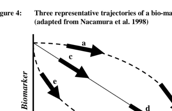
Figure 4: Three representative trajectories of a bio-marker of aging (adapted from Nacamura et al. 1998)

Note: We can see that a bio-marker of aging accelerates (ab), decelerates (ef), or assumes linearity (cd) with age in an organism. Correspondingly, the rate of aging, defined as the rate of change in the bio-marker, increases (in case of ab), decreases (in case of ef), or does not change (in case of cd) with age, depending on a variable chosen as the bio-marker of aging.

Equally, the rate of age-related changes in a bio-marker of aging (i.e., the rate of aging per se) may increase, decrease, or not change at all with age (see comment on Fig. 4). This means that at the same time, and in the same organism, the rate of aging can be characterized by increasing, decreasing, or constant functions, depending on the index chosen as the bio-marker of aging.

Does this mean that all attempts to calculate individual aging rates as a universal index are useless? In some sense, yes. First, the rate of individual aging is not an obligatory constant during life. It may change in an individual with age (as shown by the curves “ab” and “ef” in Fig. 4). Second, the aging phenotype results from age-related changes in an organism. These changes are often discordant (because the dynamics of separate age-related processes may be accelerated, decelerated, linear, or even wave-like). The relative contribution of these processes to the age phenotype may differ in individuals, creating significant variability in aging manifestations. For

b

c

d

e

f

a

A

g

ing B

iomar

ker

(16)

instance, some individuals look younger but are more vulnerable to disease than their peers, while others look older but are more resistant to acute stress, and as result live longer. What can we do, then, to study the rate of aging under such conditions? A solution is to subdivide individual aging into processes that show different age-related dynamics, and then to study these processes separately. Ukraintseva and Yashin (2001) applied this approach to explain patterns of age-specific morbidity in human populations. The authors divided all age-associated changes in an organism into three categories (basal, ontogenetic, and exposure-related) characterized by the decelerated, wave-like, and accelerated change in physiological indices with age, respectively, and showed that these have a different (sometimes even opposite) influence on age-specific risks of common diseases, including cancer (see also Ukraintseva and Yashin 2003).

(17)

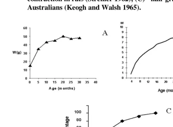
Fig. 5: Examples of a change in a bio-marker of aging at a slower rate with age: (A) - age-related change in the weight of ad libitum fed mice (Sohal and Weindruch 1996); (B) - age-related change of tail collagen contraction in rats (Strehler 1962); (C) - hair graying among 3872 Australians (Keogh and Walsh 1965).

4.3 Revised Strehler and Mildvan Model

(18)

( )

Bx

e

V

x

V

=

₀ − (4)

and the respective “rate of individual aging”, r(x), can be defined as

( )

dx

x

dV

x

r

=

−

=

V

₀

Be

−Bx

.

(5)

Note that in the revised model, “the rate of aging” r(x) =

V

₀

Be

−Bx changes as the individual progresses in years, while in the original SM model, “the rate of aging”, r(x) = V0B, is constant during the individual’s entire life.

In the original SM model, parameter B characterizes the slope of the vitality curve. In the revised model, parameter B can be interpreted as the “logarithmic rate of aging” because

( )

(

log

( )

)

( )

1

_{( )}

( )

_{( )}

.

log

B

x

V

x

r

x

V

dx

x

dV

dx

x

V

d

x

r

=

−

=

−

=

(6)

In the revised model, parameter B characterizes the slope of the logarithmic vitality curve, log V(x), and the incidence rate is

( )

D

Bx e V

Ke

x

ε

µ

− −

=

0

(7)

or, defined through the individual “rate of aging”, r(x),

( )

B

x r D

Ke

x

ε

µ

) ( −

=

.

(8)

4.4 Applying a revised Strehler and Mildvan Model to cancer data

(19)

economic progress. In particular, the overall cancer incidence rate is commonly higher in the more developed countries. Usual explanations of this association involve improved diagnostics and increased exposure to environmental carcinogens (e.g., smoking and industrial pollution). Others concentrate on rising individual vulnerability to cancer and attribute improved medical and living conditions as well as better hygiene, among others factors, to this increase; these factors are seen to favor the “relaxation” of differential selection in a population and to increase the survival of frail individuals in a population.

The revised SM model also explains the decrease in the overall cancer incidence rate at old ages (usually after 75) that is widely observed in epidemiological (both period and cohort) data. There are two different methods to obtain the declining rates.

First, we can obtain from this model the observed decline at oldest old ages and acceleration in the rates over time, assuming age-dependent parameter K (or, alternatively, parameter

ε

D) and/or age-dependent parameter B. We formulate three

modifications to the model (7):

a) Let the intensity of stress events be constant until some age T and after this age it starts to decline exponentially (as a manifestation of an older individual tending to avoid stresses):

( )

₍ ₎







>

≤

=

₋ ₋

T

x

Ke

T

x

K

T

x

K

_c _x _T

K

_,

,

(9)

where

0 <

C

_K

<<

1

. Let r(x)=B be constant. We will refer to model (7) with modification (9) as Model 1 throughout the text.

b) Assume that the intensity of stress events is constant at all ages but that the “logarithmic rate of aging” is changing over age. Assume, for instance, that this rate is constant until some age T and then it starts to decline exponentially (as a more pronounced manifestation of the basal component of aging, see Ukraintseva and Yashin 2001):

( )

₍ ₎







>

≤

=

₋ ₋

T

x

Be

T

x

B

T

x

B

_c _x _T

B

_,

,

(10)

where

0 <

C

B

<<

1

_{. We will refer to model (7) with modification (10) as}

(20)

c) Suppose that the intensity of stress events is modeled in the same way as in a.) but that at the same time the “logarithmic rate of aging” starts to increase exponentially:

( )

₍ ₎







>

≤

=

₋ ₋

T

x

Ke

T

x

K

T

x

K

_c _x _T

K

_,

,

(11)

( )

₍ ₎







>

≤

=

₋

T

x

Be

T

x

B

T

x

B

_c _x _T

B

_,

,

(12)

where

0 <

C

K

<<

1

_and

0 <

C

B

<<

1

_{. We will refer to model (7) with}

modification (11)-(12) as Model 3 throughout the text

.

In all variants of the model, the resulting incidence rates decline at old ages. Second, the observed dynamics of cancer incidence rates can also be obtained with the aging-independent parameters of the revised SM model, using a different approach. For this purpose, we include not only an exponentially decreasing rate of aging during life r(x) but also a factor of population heterogeneity, assuming variability in parameter K. The advantage of such an approach is that it allows us to consider both phenomena, a decrease in the individual rate of living with age and differential selection in a heterogeneous population within the framework of one model, explaining the decline in the overall cancer incidence rate at old ages.

To describe heterogeneity, suppose that each individual during his or her life has a specific value of intensity of stress events, denoted by K, and that this intensity is gamma distributed with mean 1 and variance

σ

2. Assume that the other parameters of the revised SM model are deterministic. Then, the conditional incidence rate of such an individual is

(

)

D

Bx e V

Ke

K

x

ε

µ

− −

=

0

|

,

(13)

and, according to the well-known formula for the gamma-frailty model (Vaupel et al. 1979), the observed incidence rate in the population is

( )

_{( )}

,

1

2 ₀

(21)

where D Bx e V

e

x ε

µ

−

=

0

) (

0 and

( )

=

∫

( )

x

dt t x

M

0 0

0 µ . We will refer to this model as Model 4 throughout the text.

5. Results

(22)

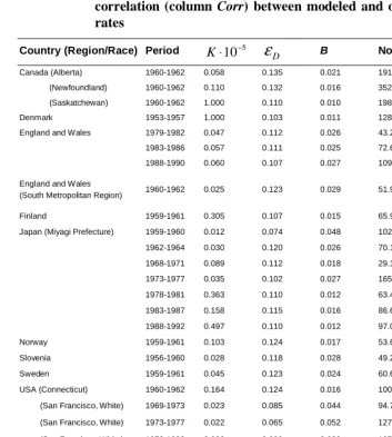
Table 1: Revised SM model with changing parameter B (Model 1) applied to data on female cancer incidence in different countries: estimations of parameters K,

ε

_D and B, norm of differences (column Norm) and correlation (column Corr) between modeled and observed incidence rates

Country (Region/Race) Period 5 10−

⋅

K

ε

D B Norm Corr

Canada (Alberta) 1960-1962 0.058 0.135 0.021 191.969 0.995

(Newfoundland) 1960-1962 0.110 0.132 0.016 352.533 0.988

(Saskatchewan) 1960-1962 1.000 0.110 0.010 198.469 0.997

Denmark 1953-1957 1.000 0.103 0.011 128.982 0.999

England and Wales 1979-1982 0.047 0.112 0.026 43.206 1.000

1983-1986 0.057 0.111 0.025 72.608 1.000

1988-1990 0.060 0.107 0.027 109.496 0.999

England and Wales

(South Metropolitan Region) 1960-1962 0.025 0.123 0.029 51.960 1.000

Finland 1959-1961 0.305 0.107 0.015 65.901 1.000

Japan (Miyagi Prefecture) 1959-1960 0.012 0.074 0.048 102.150 0.997

1962-1964 0.030 0.120 0.026 70.197 0.999

1968-1971 0.089 0.112 0.018 29.176 1.000

1973-1977 0.035 0.102 0.027 165.986 0.996

1978-1981 0.363 0.110 0.012 63.448 0.999

1983-1987 0.158 0.115 0.016 86.654 0.999

1988-1992 0.497 0.110 0.012 97.018 0.999

Norway 1959-1961 0.103 0.124 0.017 53.642 1.000

Slovenia 1956-1960 0.028 0.118 0.028 49.262 1.000

Sweden 1959-1961 0.045 0.123 0.024 60.639 1.000

USA (Connecticut) 1960-1962 0.164 0.124 0.016 100.404 0.999

(San Francisco, White) 1969-1973 0.023 0.085 0.044 94.760 0.999

(New York State) 1959-1961 0.078 0.123 0.020 65.764 1.000

(New York State) 1969-1971 0.051 0.119 0.024 60.194 1.000

(New York State) 1973-1977 0.063 0.126 0.023 173.026 0.998

(New York State) 1978-1982 0.036 0.095 0.034 46.124 1.000

(New York State) 1983-1987 0.062 0.102 0.028 42.899 1.000

(23)

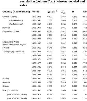
Table 2: Revised SM model with changing parameter B (Model 1) applied to data on male cancer incidence in different countries: estimations of parameters K,

ε

D and B, norm of differences (column Norm) and

correlation (column Corr) between modeled and observed incidence rates

Country (Region/Race) Period 5

10−

⋅

K

ε

D B Norm Corr

Canada (Alberta) 1960-1962 0.137 0.077 0.025 85.393 1.000

(Newfoundland) 1960-1962 1.000 0.083 0.015 175.655 0.999

(Saskatchewan) 1960-1962 0.140 0.069 0.029 116.747 1.000

Denmark 1953-1957 0.109 0.071 0.028 73.549 1.000

1983-1986 0.097 0.044 0.039 90.614 1.000

1988-1990 0.409 0.063 0.025 91.954 1.000

England and Wales

Finland 1959-1961 0.046 0.039 0.048 92.821 1.000

1962-1964 0.113 0.074 0.027 125.413 0.999

1968-1971 0.063 0.050 0.037 132.290 0.999

1973-1977 0.107 0.059 0.031 77.651 1.000

1978-1981 0.047 0.043 0.044 139.066 0.999

1983-1987 0.070 0.051 0.039 67.173 1.000

1988-1992 0.061 0.044 0.043 92.723 1.000

Norway 1959-1961 0.158 0.061 0.027 85.852 1.000

Slovenia 1956-1960 0.022 0.020 0.066 100.662 0.999

Sweden 1959-1961 0.059 0.047 0.039 95.218 1.000

USA (Connecticut) 1960-1962 0.071 0.048 0.041 122.441 1.000

(New York State) 1959-1961 0.071 0.059 0.036 75.361 1.000

(New York State) 1969-1971 0.092 0.054 0.035 75.385 1.000

(New York State) 1973-1977 0.361 0.069 0.024 183.061 0.999

(New York State) 1978-1982 0.118 0.053 0.035 100.591 1.000

(New York State) 1983-1987 0.289 0.066 0.026 72.377 1.000

(24)

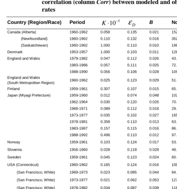
Table 3: Revised SM model with changing parameter K (Model 2) applied to data on female cancer incidence in different countries: estimations of parameters K,

ε

Country (Region/Race) Period 5

10−

⋅

K

ε

D B Norm Corr

Canada (Alberta) 1960-1962 0.058 0.135 0.021 152.586 0.997

(Newfoundland) 1960-1962 0.110 0.132 0.016 352.533 0.988

(Saskatchewan) 1960-1962 1.000 0.110 0.010 198.469 0.997

Denmark 1953-1957 1.000 0.103 0.011 128.982 0.999

1983-1986 0.057 0.111 0.025 72.608 1.000

1988-1990 0.056 0.106 0.028 109.742 0.999

England and Wales

Finland 1959-1961 0.307 0.107 0.015 65.901 1.000

1962-1964 0.030 0.120 0.026 70.197 0.999

1968-1971 0.089 0.112 0.018 29.177 1.000

1973-1977 0.035 0.102 0.027 165.986 0.996

1978-1981 0.358 0.110 0.013 63.448 0.999

1983-1987 0.157 0.115 0.016 86.654 0.999

1988-1992 0.496 0.110 0.012 97.018 0.999

Norway 1959-1961 0.103 0.124 0.017 53.642 1.000

Slovenia 1956-1960 0.028 0.118 0.028 49.262 1.000

Sweden 1959-1961 0.045 0.123 0.024 60.639 1.000

USA (Connecticut) 1960-1962 0.165 0.124 0.016 100.404 0.999

(New York State) 1959-1961 0.078 0.123 0.020 65.764 1.000

(New York State) 1969-1971 0.051 0.119 0.024 60.194 1.000

(New York State) 1973-1977 0.063 0.126 0.023 173.026 0.998

(New York State) 1978-1982 0.036 0.095 0.034 46.124 1.000

(New York State) 1983-1987 0.062 0.102 0.028 46.894 1.000

(25)

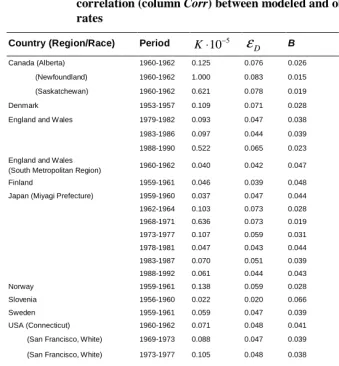
Table 4: Revised SM model with changing parameter K (Model 2) applied to data on male cancer incidence in different countries: estimations of parameters K,

ε

10−

⋅

K

ε

D B Norm Corr

Canada (Alberta) 1960-1962 0.125 0.076 0.026 81.041 1.000

(Newfoundland) 1960-1962 1.000 0.083 0.015 175.655 0.999

(Saskatchewan) 1960-1962 0.621 0.078 0.019 82.233 1.000

Denmark 1953-1957 0.109 0.071 0.028 73.549 1.000

1983-1986 0.097 0.044 0.039 90.614 1.000

1988-1990 0.522 0.065 0.023 100.755 1.000

England and Wales

Finland 1959-1961 0.046 0.039 0.048 97.569 1.000

1962-1964 0.103 0.073 0.028 126.693 0.999

1968-1971 0.636 0.073 0.019 92.801 1.000

1973-1977 0.107 0.059 0.031 77.651 1.000

1978-1981 0.047 0.043 0.044 139.066 0.999

1983-1987 0.070 0.051 0.039 67.173 1.000

1988-1992 0.061 0.044 0.043 92.723 1.000

Norway 1959-1961 0.138 0.059 0.028 81.403 1.000

Slovenia 1956-1960 0.022 0.020 0.066 100.662 0.999

Sweden 1959-1961 0.059 0.047 0.039 95.218 1.000

USA (Connecticut) 1960-1962 0.071 0.048 0.041 122.441 1.000

(New York State) 1959-1961 0.104 0.067 0.030 74.717 1.000

(New York State) 1969-1971 0.092 0.054 0.035 75.385 1.000

(New York State) 1973-1977 0.068 0.037 0.046 257.278 0.999

(New York State) 1978-1982 0.118 0.053 0.035 100.591 1.000

(New York State) 1983-1987 0.289 0.066 0.026 72.377 1.000

(26)

Table 5: Revised SM model with changing parameters B and K (Model 3) applied to data on female cancer incidence in different countries: estimations of parameters K,

ε

D and B, norm of differences (column

Norm) and correlation (column Corr) between modeled and observed

incidence rates

10−

⋅

K

ε

D B Norm Corr

Canada (Alberta) 1960-1962 0.058 0.135 0.021 152.586 0.997

(Newfoundland) 1960-1962 0.018 0.082 0.042 167.098 0.997

(Saskatchewan) 1960-1962 0.122 0.133 0.016 155.432 0.998

Denmark 1953-1957 0.117 0.123 0.018 66.652 1.000

1983-1986 0.043 0.102 0.029 40.340 1.000

1988-1990 0.041 0.092 0.033 57.376 1.000

England and Wales

Finland 1959-1961 0.307 0.107 0.015 65.901 1.000

1962-1964 0.030 0.120 0.026 70.197 0.999

1968-1971 0.089 0.112 0.018 29.177 1.000

1973-1977 0.035 0.102 0.027 165.986 0.996

1978-1981 0.359 0.110 0.013 63.448 0.999

1983-1987 0.157 0.115 0.016 86.654 0.999

1988-1992 0.492 0.110 0.012 97.018 0.999

Norway 1959-1961 0.085 0.125 0.018 52.801 1.000

Slovenia 1956-1960 0.031 0.120 0.027 48.530 1.000

Sweden 1959-1961 0.045 0.123 0.024 60.639 1.000

USA (Connecticut) 1960-1962 0.090 0.125 0.020 88.062 1.000

(New York State) 1959-1961 0.043 0.118 0.026 56.034 1.000

(New York State) 1969-1971 0.051 0.119 0.024 60.194 1.000

(New York State) 1973-1977 0.026 0.089 0.040 49.378 1.000

(New York State) 1978-1982 0.033 0.091 0.036 43.516 1.000

(New York State) 1983-1987 0.062 0.102 0.028 46.894 1.000

(27)

Table 6: Revised SM model with changing parameters B and K (Model 3) applied to data on male cancer incidence in different countries: estimations of parameters K,

ε

_D and B, norm of differences (column

Norm) and correlation (column Corr) between modeled and observed

incidence rates

10−

⋅

K

ε

D B Norm Corr

Canada (Alberta) 1960-1962 0.133 0.077 0.025 73.954 1.000

(Newfoundland) 1960-1962 0.042 0.059 0.039 134.202 0.999

(Saskatchewan) 1960-1962 0.769 0.079 0.018 74.564 1.000

Denmark 1953-1957 0.077 0.063 0.032 63.769 1.000

1983-1986 0.138 0.052 0.033 86.959 1.000

1988-1990 0.525 0.066 0.023 100.755 1.000

England and Wales

Finland 1959-1961 0.046 0.039 0.048 97.569 1.000

1962-1964 0.103 0.073 0.028 126.693 0.999

1968-1971 1.000 0.073 0.017 66.644 1.000

1973-1977 0.107 0.059 0.031 77.651 1.000

1978-1981 1.000 0.079 0.016 87.701 1.000

1983-1987 0.110 0.062 0.032 44.426 1.000

1988-1992 0.075 0.051 0.039 86.862 1.000

Norway 1959-1961 0.167 0.062 0.026 77.042 1.000

Slovenia 1956-1960 0.024 0.024 0.061 98.582 0.999

Sweden 1959-1961 0.059 0.046 0.039 95.218 1.000

USA (Connecticut) 1960-1962 0.071 0.048 0.041 122.441 1.000

(New York State) 1959-1961 0.108 0.068 0.030 65.152 1.000

(New York State) 1969-1971 0.107 0.057 0.033 73.660 1.000

(New York State) 1973-1977 1.000 0.075 0.018 203.271 0.999

(New York State) 1978-1982 0.286 0.068 0.025 93.045 1.000

(New York State) 1983-1987 0.395 0.068 0.024 69.551 1.000

(28)

Table 7: Revised SM model with heterogeneity in parameter K (Model 4) applied to data on female cancer incidence in different countries: estimations of parameters

σ

2,

ε

_D and B, norm of differences (column Norm) and correlation (column Corr) between modeled and observed incidence rates

Country (Region/Race) Period

σ

2

ε

_D B Norm Corr

Canada (Alberta) 1960-1962 4.871 0.087 0.016 371.808 0.981

(Newfoundland) 1960-1962 0.359 0.111 0.010 360.808 0.987

(Saskatchewan) 1960-1962 1.769 0.099 0.013 396.752 0.987

Denmark 1953-1957 0.816 0.098 0.013 259.680 0.996

1983-1986 1.121 0.100 0.012 101.505 0.999

1988-1990 1.077 0.099 0.013 139.143 0.999

England and Wales

Finland 1959-1961 1.786 0.089 0.014 113.617 0.999

1962-1964 8.503 0.074 0.018 304.107 0.977

1968-1971 4.122 0.083 0.014 129.228 0.997

1973-1977 3.504 0.084 0.014 154.502 0.996

1978-1981 4.799 0.081 0.015 190.424 0.994

1983-1987 3.248 0.086 0.014 153.448 0.997

1988-1992 2.622 0.092 0.013 166.928 0.997

Norway 1959-1961 1.051 0.102 0.011 61.494 1.000

Slovenia 1956-1960 5.252 0.086 0.015 145.189 0.996

Sweden 1959-1961 4.112 0.087 0.015 194.733 0.995

USA (Connecticut) 1960-1962 0.494 0.107 0.011 111.439 0.999

(New York State) 1959-1961 1.654 0.098 0.013 117.910 0.999

(New York State) 1969-1971 1.988 0.097 0.013 82.540 0.999

(New York State) 1973-1977 0.840 0.108 0.011 207.190 0.998

(New York State) 1978-1982 1.803 0.095 0.014 68.730 1.000

(New York State) 1983-1987 2.654 0.084 0.017 101.588 0.999

(29)

Table 8: Revised SM model with heterogeneity in parameter K (Model 4) applied to data on male cancer incidence in different countries: estimations of parameters

σ

2,

ε

_D and B, norm of differences (column Norm) and correlation (column Corr) between modeled and observed incidence rates

Country (Region/Race) Period

σ

2

ε

_D B Norm Corr

Canada (Alberta) 1960-1962 2.683 0.061 0.021 110.189 1.000

(Newfoundland) 1960-1962 1.624 0.066 0.020 337.911 0.996

(Saskatchewan) 1960-1962 1.283 0.063 0.021 130.952 1.000

Denmark 1953-1957 1.641 0.064 0.020 204.059 0.998

1983-1986 1.107 0.057 0.023 83.649 1.000

1988-1990 0.703 0.062 0.022 149.752 1.000

England and Wales

Finland 1959-1961 2.397 0.058 0.024 80.926 1.000

1962-1964 6.596 0.033 0.033 398.346 0.987

1968-1971 4.108 0.040 0.028 273.474 0.996

1973-1977 2.912 0.042 0.027 388.519 0.995

1978-1981 3.285 0.047 0.026 252.474 0.997

1983-1987 2.174 0.053 0.024 194.626 0.999

1988-1992 1.948 0.055 0.024 166.106 0.999

Norway 1959-1961 2.170 0.058 0.021 73.705 1.000

Slovenia 1956-1960 6.482 0.036 0.031 281.685 0.993

Sweden 1959-1961 3.324 0.045 0.026 227.656 0.998

USA (Connecticut) 1960-1962 1.174 0.065 0.021 138.767 1.000

(New York State) 1959-1961 1.541 0.066 0.020 66.905 1.000

(New York State) 1969-1971 2.041 0.051 0.025 226.711 0.999

(New York State) 1973-1977 0.866 0.067 0.021 277.710 0.999

(New York State) 1978-1982 1.187 0.056 0.024 175.271 1.000

(New York State) 1983-1987 1.571 0.044 0.028 399.447 0.998

(30)

The four models provide an adequate fit to the data in different regions and time periods. Norms of differences and correlations between modeled and observed incidence rates for the same data set in Models 1-3 are comparable (see columns Norm and Corr in Tables 1-8). Model 3 has greater flexibility because it has an additional parameter and is capable of producing a better fit for some data sets. Model 4 fit least according to the norms of differences and correlations between modeled and observed incidence rates. Nevertheless, all four models capture the observed patterns of cancer incidence rates (except a peak in early childhood): a low rate in youth, an increase in this rate during adolescence, and a deceleration or decline at old ages. The models also produce non-declining rates when parameter T equals the maximal age of available data (85) or parameters cB or cK are zeros.

Estimations of parameters

ε

D and B for the same data set are similar in Models

1-3 in most cases. This is a predictable result because the models have, in essence, the same incidence rate until age T and then differ either in the slope of the “vitality” function or the intensity of stress events in age interval [T, 85]. The estimations, however, show variability between different data sets, reflecting substantial variability between the observed rates in different countries and changes in the rates over time in the same country. For instance, the Miyagi prefecture incidence rates at oldest old ages almost doubled 1950-1990s (Fig. 1). Parameters

ε

_D, B and K define the patterns of incidence rates and, therefore, are also subject to variability over time and place. The models are less sensitive to changes in parameter K and, in some cases, this parameter varies to a greater extent in Models 1-3 and in different data sets within the same model. We restricted the parameter K to be less than 105 in our models. In some cases, the estimations of K reach the upper boundary, but the greater values of K would result only in a minor improvement of fit. We also assumed T to be greater than 70 (around the minimal age of decline in the incidence rates) and the estimations are at boundary in some cases. However, a further reduction of the lower boundary gives no substantial improvement of fit.

(31)

The models with a constant “logarithmic rate of aging” B over age (Model 1), a decreasing B at oldest ages (Model 2) and an increasing B at oldest ages (Model 3) result in declining patterns of cancer incidence rates. This means that the observed decline in the rates may be the result of three different dynamics of the “logarithmic rates of aging” and intensities of stress events related to cancer. We interpret these changes as a more pronounced manifestation of the basal component of aging within the context of Ukraintseva and Yashin’s (2001) model. The logarithmic rate of aging possibly does not change with age, in contrast to the intensity. We can also assume that the intensity is fixed over age, whereas the logarithmic rate of aging declines at oldest old ages. As a variation of the first model, we can assume that the declining intensity at advanced ages is accompanied by an increasing logarithmic rate of aging. Note that we can alternatively impose changes on the average amplitude of stress events

ε

D rather

than intensity K.

Male and female cancer incidence rates are different. Males have higher incidence rates at older ages than the opposite sex. The stable relationship between the estimations of parameters B and

ε

_D for male and female data in Model 4 reflects this observation. The resulting estimates of

ε

_D are higher for females in all data sets, while the estimates of B are always higher for males (see Tables 7-8). A trade-off between resource allocation strategies in the male and female organisms, i.e., between average amplitudes of stress events and the rates of physiological aging, possibly explains this phenomenon. The female organism spends a greater part of her resources on “protection” against physiological aging. As a result, the values of B are lower and that of

ε

_D are higher. The male organism, on the contrary, “fights” harmful influences and therefore reduces the amplitude of stress events that “reach” the organism. Thus, the corresponding parameters

ε

_D are lower than that of females, but the trade-off is the higher rate of physiological aging B.

The observed increase in cancer incidence rates over time can be obtained in Models 1-4 if, for instance, one of the parameters

ε

_D and B is increasing and the second is constant or declining. Then, changes in parameters

ε

D and B over time can

(32)

6. Conclusion

The literature on mathematical models of carcinogenesis is vast; see e.g., the works by Yakovlev and Tsodikov (1996) and Moolgavkar et al. (1999), a recent review paper by van Leeuwen and Zonneveld (2001) and references in these works. In this paper, we mentioned several very specific mathematical models only, and they had been “selected” to explain observed trends in overall cancer incidence rates. We also analyzed data on cancer incidence rates in different regions at different periods, applying the revised SM model (both with age-dependent parameters and with heterogeneity). These models suggest different reasons for the observed patterns of overall cancer incidence rates. The analyses of the models demonstrate that:

1) The observed decline in overall human cancer incidence rates at old ages can be a pronounced manifestation of the basal component of individual aging. This result can be obtained by a decline (over age) in the related parameter of the logarithmic rate of aging (parameter B in Model 2) or by an age-related decline in intensity of external stresses at old ages (parameter K in Model 1).

2) Effects of population heterogeneity in the susceptibility to external stresses can also explain this decline (Model 4). In this model, differences in values of variance of the heterogeneity distribution explain differences in the rates of decline at old ages observed in different populations and time periods.

3) The models are capable of explaining the interesting phenomenon observed in the overall cancer incidence rates, namely the intersection of male/female rates. This universal pattern may be a result of different resource allocation strategies (“fighting” external stresses and “fighting” physiological aging) that are used by the male and female organisms. This intriguing pattern needs further explanation, from both a biological and a mathematical perspective. Available molecular-biological and epidemiological data allow for the development of more sophisticated mathematical models of these mechanisms.

4) The observed increase in cancer incidence rates over time can be interpreted in terms of changes in the resource allocation strategies over time (i.e., resource allocation between “fighting” external stresses and “fighting” physiological aging). Over-time trends in parameters of Models 1-4 (when one of the parameters

ε

_D or B is increasing and the second is constant or declining over time) can reflect this phenomenon.

(33)

time-series data on changes in stress-resistance with age (e.g., cellular sensitivity to oxidative stress). This permits associations to be made between the unspecified physiological index (“vitality”) and real physiological parameters. Applications of various models that incorporate the observed physiological parameters to large time series data on human morbidity and mortality can help to obtain deeper insights into the possible mechanisms that regulate aging-related changes in the physiological parameters, elucidate various factors responsible for the modification of the respective patterns over time and target appropriate prophylaxis to reduce physiological decline.

In this paper, we focused mainly on biological explanations of observed declines in the age-trajectories of human cancer incidence rates. This does not mean that other explanations should not be taken into account. The dynamics of age-specific cancer incidence rates over time reflects the combined influence of various factors (social, behavioral, environmental, medical etc.). The possible causes of this decline include: (i) the effects of cross-sectional data that transform cohort dynamics into age patterns, (ii) population heterogeneity that selects individuals susceptible to cancer, (iii) a decline in some carcinogenic exposures in older individuals, (iv) underdiagnostics in older people – it leads to a smaller detection number of new cases existing latently, and (v) the effects of individual aging that slow down major physiological processes in an organism. None of these factors can be neglected. The first four causes have been discussed in the literature to some extent. Our present paper provided some new insights into possible biological explanations for the observed phenomena. More elaborated models are needed to incorporate all of them and reveal the relative impact of these factors on observed trends. This would provide the grounds for fruitful discussions and stimulate further research directions. Changes in social, behavioral, environmental, and medical conditions would induce changes in internal (molecular-biological) mechanisms that are responsible for cancer development. If a convincing rationale is available for representing a disease etiology in a specific mathematical model, it should not to be ignored in data analysis.

7. Acknowledgements

(34)

References

Anstey K.J., Lord S.R., Smith G.A. (1996). “Measuring human functional age: a review of empirical findings”. Exp. Aging Res., 22, 3: 245-266.

Armitage P., Doll R. (1954). “The age distribution of cancer and a multistage theory of carcinogenesis”. Br. J. Cancer, 8: 1-12.

Benson D., Mitchell N., Dix D. (1996). “On the role of aging in carcinogenesis”. Mutation Research/Fundamental and Molecular Mechanisms of Mutagenesis, 356, 2: 209-216.

Cheron G., Desmedt J.E. (1980). “Peripheral and central somatosensory pathways and evoked cerebral potentials during aging”. Rev. Electroencephalogr. Neurophysiol. Clin., 10: 146-152.

Dean W. (1988). Biological Aging Measurement. Los Angeles: The Center Biogerontol. Dix D. (1989). “The role of aging in cancer incidence: an epidemiological study”. J.

Gerontol., 44, 6: 10-18.

Grove G., Kilgman A. (1983). “Age-associated changes in human epidermal cell renewal”. J. Geront., 38: 137-142.

Guyton A.C., Hall J.E. (1996). Textbook of Medical Physiology. Philadelphia: W.B. Saunders Co.

Health US, DHHS Publications, 1997-2000.

IARC (1965). Cancer Incidence in Five Continents. Volume I. Lyon: International Agency for Research on Cancer.

IARC (1970). Cancer Incidence in Five Continents. Volume II. Lyon: International Agency for Research on Cancer.

IARC (1976). Cancer Incidence in Five Continents. Volume III. Lyon: IARC Sci Publ, 15.

IARC (1982). Cancer Incidence in Five Continents. Volume IV. Lyon: IARC Sci Publ, 42.

IARC (1987). Cancer Incidence in Five Continents. Volume V. Lyon: IARC Sci Publ, 88.

(35)

IARC (1997). Cancer Incidence in Five Continents. Volume VII. Lyon: IARC Sci Publ, 143.

Keogh E., Walsh R. (1965). “Rate of graying of human hair”. Nature, 207: 877-878. Krtolica A., Campisi J. (2002). “Cancer and aging: a model for the cancer promoting

effects of the aging stroma”. Int. J. Biochem. Cell. Biol., 34, 11: 1401.

Kuramoto K., Matsushita S., Esaki Y., Shimada H. (1993). “Prevalence, rate of correct clinical diagnosis and mortality of cancer in 4,894 elderly autopsy cases”. Nippon Ronen Igakkai Zasshi., 30, 1: 35-40, in Japanese.

McClearn G.E. (1997). “Bio-markers of age and aging”. Exp. Gerontol., 32, 1-2: 87-94. Moolgavkar S.H., Venzon D.J. (1979). “Two-event models for carcinogenesis:

incidence curves for childhood and adult tumors”. Math. Biosci., 47: 55-77. Moolgavkar S.H., Knudson A.G. (1981). “Mutation and cancer: a model for human

carcinogenesis”. J. Natl. Cancer Inst., 66: 1037-1052.

Moolgavkar S.H., Luebeck E.G. (1990). “Two-event model for carcinogenesis: biological, mathematical and statistical considerations”. Risk Anal., 10: 323-341. Moolgavkar S.H., Krewski D., Zeise L., Cardis E., Møller H. (1999). Quantitative

Estimation and Prediction of Human Cancer Risks. Lyon: IARC Sci Publ.

Nakamura E., Lane M., Roth G., Ingram D. (1998). “A strategy for identifying bio-markers of aging”. Exp. Gerontology, 33: 4.

Peto R., Roe F.J., Lee P.N., Levy L., Clack J. (1975). “Cancer and ageing in mice and men.” Br. J. Cancer, 32, 4: 411-426.

Peto R., Parish S.E., Gray R.G. (1985). “There is no such thing as ageing, and cancer is not related to it”. IARC Sci Publ, 58: 43-53.

Pompei F., Polkanov M., Wilson R. (2001). “Age distribution of cancer in mice: the incidence turnover at old age.” Toxicol Ind Health, 17, 1: 7-16.

Rainsford J., Cohen P., Dix D. (1985). “On the role of aging in cancer incidence: analysis of the lung cancer data”. Anticancer Res, 5, 4: 427-430.

(36)

Riggs J.E., Millecchia R.J. (1992). “Using the Gompertz-Strehler Model of Aging and Mortality to Explain Mortality Trends in Industrialized Countries”. Mechanisms of Aging and Development, 65: 217-228.

Riggs J.E., Hobbs G.R. (1998). “Nonrandom sequence of slope-intercept estimates in longitudinal Gompertzian analysis suggests biological relevance”. Mechanisms of Aging and Development, 100: 269-275.

Robertson C., Gandini S., Boyle P. (1999). “Age-Period-Cohort Models: A Comparative Study of Available Methodologies”. J Clin Epidemiol, 52, 6: 569-583.

Rubin H. (1997). “Cell aging in vivo and in vitro”. Mech. Aging and Dev., 98: 1-35. Smith D. (1996). “Cancer mortality at very old ages”. Cancer, 77, 7: 1367-1372. Smith D. (1999). “Resistance to causes of death: a study of cancer mortality resistance

in the oldest old”. In: Robine J-M et. al. (Eds). The Paradoxes of Longevity. Springer-Verlag: 61-71.

Sohal R., Weindruch R. (1996). “Oxidative stress, caloric restriction, and aging”. Science, 273: 59-63.

Stanta G., Campagner L., Cavallieri F., Giarelli L. (1997). “Cancer of the oldest old. What we have learned from autopsy studies.” Clin Geriatr Med., 13, 1: 55-68. Strehler B. (1962). Time, Cells, and Aging. London: Academic Press.

Strehler B.L., Mildvan A.S. (1960). “General theory of mortality and aging”. Science, 132: 14-21.

Ukraintseva S.V., Yashin A.I. (2001). “How individual aging may influence human morbidity and mortality patterns”. Mech. Aging and Dev., 122: 1447-1460. Ukraintseva S.V., Yashin A.I. (2003). “Individual aging and cancer risk: How are they

related?” Demographic Research, 9, 8: 163-196.

Van Leeuwen I.M.M., Zonneweld C. (2001). “From exposure to effect: a comparison of modeling approaches to chemical carcinogenesis”. Mutation Research, 489: 17-45.

Vaupel J.W., Manton K.G., Stallard E. (1979). “The impact of heterogeneity in individual frailty on the dynamics of mortality”. Demography, 16: 439-454. Vaupel J.W., Yashin A.I. (1985). “Heterogeneity’s ruses: some surprising effects of

(37)

Vaupel J.W., Yashin A.I. (1988). “Cancer Rates over Age, Time, and Place: Insights from Stochastic Models of Heterogeneous Populations.” WP #88-01-1 of the Center for Population Analysis and Policy, University of Minnesota, and MPIDR Working Paper WP 1999-006.

Volpe E.W., Dix D. (1986). “On the role of aging in cancer incidence: cohort analyses of the lung cancer data”. Anticancer Res, 6, 6: 1417-1420.

Yakovlev A.Yu., Asselain B., Bardou V.-J., Fourquet A., Hoang T., Rochefodiere A., Tsodikov A.D. (1993). “A simple stochastic model of tumor recurrence and its application to data on pre-menopausal breast cancer”. In: Asselain B., Boniface M., Duby C., Lopez C., Masson J.P., Tranchefort J., editors. Biometrie et Analyse de Donnees Spatio-Temporelles No 12. Rennes: Societe Francaise de Biometrie, ENSA Rennes, France: 66-82.

(38)