An efficient approximate method for solution of the heat equation using Laguerre-Gaussians radial functions

(1)

An eﬃcient approximate method for solution of the heat equation

using Laguerre-Gaussians radial functions

M. Khaksarfard

Department of Mathematics, Faculty of Mathematical Sciences, Alzahra University, Tehran, Iran.

E-mail: [email protected]

Y. Ordokhani∗

Department of Mathematics, Faculty of Mathematical Sciences, Alzahra University, Tehran, Iran.

E. Babolian

Faculty of Mathematical Sciences and Computer, Kharazmi University, Tehran, Iran.

Abstract In the present paper, a numerical method is considered for solving one-dimensional heat equation subject to both Neumann and Dirichlet initial boundary conditions. This method is a combination of collocation method and radial basis functions (RBFs). The operational matrix of derivative for Laguerre-Gaussians (LG) radial basis functions is used to reduce the problem to a set of algebraic equations. The re-sults of numerical experiments are presented to conﬁrm the validity and applicability of the presented scheme.

Keywords. Radial basis functions, Heat conduction, Dirichlet and Neumann boundary Conditions.

2010 Mathematics Subject Classification. 65M99, 35K20.

1. _Introduction

Partial diﬀerential equations have a wide range of applications in chemistry and physics. Theory and numerical schemes for solving initial boundary value problems have attracted the attention of researchers. Youseﬁ proposed Bernstein Tau tech-nique to solve the one-dimensional parabolic equation in [22] and Tohidi presented the solution of this problem by the Legendre collocation method in [17]. Numerical solutions of parabolic equation with an initial-boundary value problem that combines Neumann and Dirichlet conditions were investigated in [1,2,3,4,5,21]. The general form of equation is given as:

ut(x, t) =uxx(x, t) +Q(x, t), 0< x < L,0< t≤T, (1.1) with the initial condition:

u(x,0) =f(x), 0≤x≤L, (1.2)

Received: 21 December 2016 ; Accepted: 21 February 2017. ∗Corresponding author.

(2)

and the boundary conditions

u(0, t) =g0(t), u(L, t) =g1(t), 0< t≤T, (1.3)

ux(0, t) =g2(t), ux(L, t) =g3(t), 0< t≤T, (1.4)

where Q(x, t), f(x), g0(t), g1(t), g2(t) and g3(t) are suitably given functions. He

in [9,10] and Cheniguel in [5] proposed the homotopy perturbation method (HPM) to solve initial boundary value problems. Mohebbi presented a class of new finite difference schemes to solve the one-dimensional heat and advection-diffusion equations in [13]. Sun in [16] proposed a class of new finite difference methods, CBVM, to solve the one dimension heat equations.

The organization of this article is as follow. We describe radial basis functions and their properties in Section 2. In Section 3, the use of this basis is discussed for solving one-dimensional heat equation. In Section 4, we give some computational results of numerical experiments with RBFs method to support our theoretical discussion. The conclusion is presented in Section 5.

2. _{Radial basis function approximation}

Polynomials (e.g., Legendre and Chebyshev) are very efficient tools for interpolat-ing a set of points in one-dimensional domains but in irregular domains and higher-dimensional the use of these functions is not effective. The main benefit of radial basis functions is that this method is independent of the dimension of the problem and needs neither domain nor surface discretization. The method is meshless and is not difficult.

2.1. Deﬁnition of RBF. Let R+ ₌ _{_x _∈ _R_{, x} _≥ ₀_}_, _∥_._∥

2 denotes the Euclidean

norm and φ : R+ _→ _R _{be a continuous function with} _φ(0) _≥ _{0. A radial basis}

function onRd _{is a function of the form:}

ϕi(x) =φ(∥x−xi∥2),

which depends only on the distance betweenx∈Rd _{and a ﬁxed point}_x

i ∈Rd. So that the radial basis functionϕi is radially symmetric about the centerxi.

Letx1,x2,· · · ,xN ∈Ω⊂Rdbe a given set of scattered data. A radial basis function interpolation problem may be described as:

Sf(x) = N

∑

i=1

λiϕi(x),

for given datafi=f(xi),i= 1,2,· · ·, N, whereλiare chosen in order toSf(xj) =fj, j= 1,2,· · ·, N, that the interpolation conditions provide the linear system:

Aλ=f,

where fori, j ∈ {1,2,· · ·, N},Aij=ϕi(xj),λ= [λ1, λ2,· · ·, λN]T andf = [f1, f2,· · ·, fN]T. Let r be the Euclidean distance between a ﬁxed point xi ∈ Rd and x ∈ Rd, i.e. ∥x−xi∥2. Some well-known RBFs are listed in Table 1. The kind of RBFs, we will

(3)

Table 1. Some well-known functions that generate RBFs.

Name of Radial Basis Function Deﬁnition Multiquadric(MQ) φ(r) =√ε2₊_r2

Inverse Quadratic(IQ) φ(r) = ₍_ε2₊1_r2₎ Inverse Multiquadric(IMQ) φ(r) = √ 1

ε2₊_r2 Gaussian(GA) φ(r) =e−ε2_r2 Thin Plate Splines(TPS) φ(r) =r2log(r)

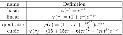
basis functions are the Mat´ern functions, also known as Sobolev splines. Examples are listed in Table 2. Another RBFs are the Laguerre-Gaussians. The deﬁnition of

Table 2. Mat´ern functions.

name Deﬁnition

basic φ(r) =e−εr linear φ(r) = (1 +εr)e−εr quadratic φ(r) = (1 +εr+(εr₃)2)e−εr

cubic φ(r) = (15 + 15εr+ 6(εr)2_{+ (εr)}3_)e−εr

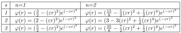
Laguerre-Gaussians functions family comes from the generalized Laguerre polynomi-als of degreenand orders/2 [14]. Speciﬁc examples are listed in Table 3.

The shape parameterε, which appears in tables affects both the accuracy of the esti-mate and the conditioning of the interpolation matrix [15]. Almost, for fixed values of the shape parameterε, the condition number increases withN. For a fixed numberN, smaller shape parameters produce more accurate approximations, but they are also associated with a poorly conditionedA. However, many researchers have attempted to develop algorithms for choosing optimal values of the shape parameter but the optimal choice of the shape parameter is still an open question and it is most often selected by brute force. Franke [7] suggestedε2= 1.25D/√N in MQ basis, whereD is the diameter of the smallest circle containing all data points andNis the number of data points. Hardy [8] recommended the use ofε2_{= 0.815d}_where_d_{= (1/N)}∑N

i=1di anddi is the distance from the data pointxi to its nearest neighbor. Recently, Forn-berg developed a Contour-Pad´e algorithm that is capable of stably computing the RBF approximation for allε >0 [6]. Micchelli [12] and Wendland [18] showed that the interpolation matrix for the RBFs is invertible for distinct interpolation points. We have the following theorem about the convergence of RBFs interpolation.

Theorem 2.1. Assume {xi}Ni=1 are N nodes inΩ⊂Rd which is convex, let:

h= max

x_∈Ω1_≤mini_≤N∥x−xi∥2,

whenϕ(η)ˆ < c(1+|η|)−2l+d, for any y satisfing∫(ˆy(η))2/ϕ(η)dη <ˆ ∞, we have:

(4)

Table 3. Laguerre-Gaussians radial functions.

s n=1 n=2

1 φ(r) = (3 2−(εr)

2_)e(−εr)2

φ(r) = (15 8 −

5 2(εr)

2₊1 2(εr)

4_)e(−εr)2

2 φ(r) = (2−(εr)2_)e(−εr)2 _{φ(r) = (3}₋_3(εr)2₊1 2(εr)

4_)e(−εr)2

3 φ(r) = (5₂−(εr)2)e(−εr)2 φ(r) = (35₈ −7₂(εr)2+1₂(εr)4)e(−εr)2

whereϕ is RBFs and the constantc depends on the RBFs, ϕˆandyˆ are supposed to be the Fourier transforms ofϕ andy respectively, y(α) _{denotes the}_α_{th derivative of}

y,yN is the RBFs approximation ofy,dis space dimension,l andαare nonnegative

integers.

Proof. A complete proof is given by authors [19,20].

2.2. Function approximation. LetX=L2_{(Ω) where Ω = [0, L]}_×_{[0, T}_{] and}

{ψ11(x, t), ..., ψ1M(x, t), ψ21(x, t), ..., ψ2M(x, t), ..., ψN1(x, t), ..., ψN M(x, t)} ⊂X be the set of LG-RBFs whereψij(x, t) = (2−ε2((x−xi)2+(t−tj)2))e−ε

2₍₍_x₋_x

i)2+(t−tj)2)

and

Y =span{ψ11(x, t), ..., ψ1M(x, t), ψ21(x, t), ..., ψ2M(x, t), ..., ψN1(x, t), ..., ψN M(x, t)}, suppose thaty be an arbitrary element inX. SinceY is a ﬁnite dimensional vector space,y has the unique best approximation out ofY asyN M ∈Y, that is [11]:

∀g∈Y,∥y−yN M∥2≤ ∥y−g∥2.

SinceyN M ∈Y, there exist unique coeﬃcientsc11, ..., c1M, c21, ..., c2M, ..., cN1, ..., cN M such that:

y≃yN M = N

∑

i=1

M

∑

j=1

cijψij(x, t) =CTΨN M(x, t) = ΨTN M(x, t)C,

whereC and ΨN M(x, t) are vectors with the form:

C= [c11, ..., c1M, c21, ..., c2M, ..., cN1, ..., cN M]T, (2.1)

ΨN M(x, t) = [ψ11(x, t), ..., ψ1M(x, t), ψ21(x, t)..., ψN M(x, t)]T. (2.2)

3. _{The operational matrix of derivative}

Letxi =L_Ni, i= 1,2, ..., N,andtj =T_Mj , j = 1,2, ..., M.The unknown function u(x, t) in (1.1)-(1.4) can be approximated as:

u(x, t) = N

∑

i=1

M

∑

j=1

cijψij(x, t) =CTΨN M(x, t). (3.1)

The diﬀerentiation with respect toxof vectors ΨN M in (2.2) can be expressed as: ∂

(5)

whereDN(x) is the operational matrix of derivative with respect toxand

ΦN M(x, t) = [ϕ11(x, t), ..., ϕ1M(x, t), ϕ21(x, t), ..., ϕN M(x, t)]T, (3.3)

where ϕij(x, t) is the GA-RBFs, i.e. ϕij(x, t) = e−ε 2₍₍_x₋_x

i)2+(t−tj)2)_{. The matrix}

DN(x) can be obtained as:

∂

∂xΨN M(x, t) =

                   

−2ε2(x−x1)(ψ11(x, t) +ϕ11(x, t))

.. .

−2ε2(x−x1)(ψ1M(x, t) +ϕ1M(x, t)) −2ε2(x−x2)(ψ21(x, t) +ϕ21(x, t))

.. . −2ε2_(x₋_x

2)(ψ2M(x, t) +ϕ2M(x, t)) ..

. −2ε2_(x₋_x

N)(ψN1(x, t) +ϕN1(x, t))

.. . −2ε2_(x₋_x

N)(ψN M(x, t) +ϕN M(x, t))

                    . (3.4)

By comparing (3.2) and (3.4), we can write:

∂

∂xΨN M(x, t) =

    

M1(x) 0 ... 0

0 M2(x) ... 0

..

. ... . .. ...

0 0 ... MN(x)

                        

ψ11(x, t) +ϕ11(x, t)

.. .

ψ1M(x, t) +ϕ1M(x, t) ψ21(x, t) +ϕ21(x, t)

.. .

ψ2M(x, t) +ϕ2M(x, t) ..

.

ψN1(x, t) +ϕN1(x, t)

.. .

ψN M(x, t) +ϕN M(x, t)

                    , (3.5)

whereMi(x) =−2ε2(x−xi)IM, i= 1,2, ..., N andIM is theM×M identity matrix. Thus we have:

DN(x) =

    

M1(x) 0 ... 0

0 M2(x) ... 0

..

. ... . .. ...

0 0 ... MN(x)

   

(6)

Similarly, the diﬀerentiation of vectors ΨN M with respect to t in (2.2) can be ex-pressed as:

∂

∂tΨN M(x, t) =DM(t)ΨN M(x, t) +DM(t)ΦN M(x, t), (3.7) whereDM(t) =diag(N1(t), N2(t), ..., NM(t)) andNi(t) =−2ε2(t−ti)IN, i= 1,2, ..., M. Also:

∂2

∂x2ΨN M(x, t) =

                   

(−2ε2_{+ (}₋_2ε2_(x₋_x

1))2)ψ11(x, t) + (−2ε2+ 2(−2ε2(x−x1))2)ϕ11(x, t)

.. . (−2ε2_{+ (}₋_2ε2_(x₋_x

1))2)ψ1M(x, t) + (−2ε2+ 2(−2ε2(x−x1))2)ϕ1M(x, t) (−2ε2+ (−2ε2(x−x2))2)ψ21(x, t) + (−2ε2+ 2(−2ε2(x−x2))2)ϕ21(x, t)

.. .

(−2ε2+ (−2ε2(x−x2))2)ψ2M(x, t) + (−2ε2+ 2(−2ε2(x−x2))2)ϕ2M(x, t) ..

. (−2ε2_{+ (}₋_2ε2_(x₋_x

N))2)ψN1(x, t) + (−2ε2+ 2(−2ε2(x−xN))2)ϕN1(x, t)

.. . (−2ε2_{+ (}₋_2ε2_(x₋_x

N))2)ψN M(x, t) + (−2ε2+ 2(−2ε2(x−xN))2)ϕN M(x, t)

                    . (3.8)

So we can write: ∂2

∂x2ΨN M(x, t) = (R+D 2

N(x))ΨN M(x, t) + (R+ 2DN2(x))ΦN M(x, t), (3.9)

where R=     

−2ε2

0 ... 0

0 −2ε2 ... 0

..

. ... . .. ...

0 0 ... −2ε2

   

 . (3.10)

Using Eqs. (3.7) and (3.9) in Eq. (1.1), we obtain:

CT_(D

M(t)−D2N(x)−R)ΨN M(x, t) +CT(DM(t)−2D2N(x)−R)ΦN M(x, t)

−Q(x, t) = 0, (3.11) and using Eqs. (3.1) and (3.2) in (1.2)-(1.4) yields:

CTΨN M(x,0)−f(x) = 0, (3.12)

CTΨN M(0, t)−g0(t) = 0, (3.13)

(7)

CTDN(0)ΨN M(0, t) +CTDN(0)ΦN M(0, t)−g2(t) = 0, (3.15)

CTDN(L)ΨN M(L, t) +CTDN(L)ΦN M(L, t)−g3(t) = 0. (3.16)

We collocate (3.11) in (N−2)×(M−1) interior points{(xl, ts)|l= 2, ..., N−1, s= 2, ..., M}, so we have:

CT(DM(ts)−DN2(xl)−R)ΨN M(xl, ts) +CT(DM(ts)−2DN2(xl)−R)ΦN M(xl, ts) −Q(xl, ts) = 0. (3.17)

Now, collocating (3.12) inN pointsxl, l= 1,2, ..., N,leads to:

CTΨN M(xl,0)−f(xl) = 0. (3.18) By collocating (3.13) and (3.14) or (3.15) and (3.16) in (M-2) pointsts, s= 2,3, ..., M, we have:

CTΨN M(0, ts)−g0(ts) = 0, (3.19)

CTΨN M(L, ts)−g1(ts) = 0, (3.20)

CTDN(0)ΨN M(0, ts) +CTDN(0)ΦN M(0, ts)−g2(ts) = 0, (3.21)

CTDN(L)ΨN M(L, ts) +CTDN(L)ΦN M(L, ts)−g3(ts) = 0, (3.22) respectively.

Eqs. (3.17)-(3.20) or Eqs. (3.17), (3.18), (3,21) and (3.22) give anN×M system of linear equations, which can be solved forcij, i= 1, ..., N, j= 1, ..., M.

4. Numerical examples

In this section we give some computational results of numerical experiments with the method based on the preceding sections, to support our theoretical discussion. In the process of computation, all the symbolic and numerical computations were performed using Maple and shape parameters were chosen by trial and error. The readers can see the eﬃciency of the proposed method from the provided ﬁgures and tables in the following examples.

Example 1. Consider Eqs. (1.1)-(1.4) withL= 1, T = 1 and [17,22]

Q(x, t) = (π2+ 1)etsin(πx), (4.1)

f(x) = sin(πx), g0(t) = 0, g1(t) = 0, (4.2)

with the exact solution

(8)

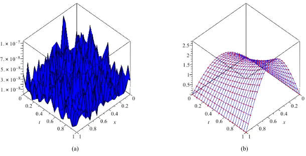
Table 4. Absolute values of error for u from Example 1.

(x, t) Method [17] Method [22] Present method

M=N=10, ε=0.6 M=N=16,ε=0.8 (0.1,0.1) 2.3106E–06 7.8747E–05 8.1463E–07 6.5626E–08 (0.2,0.2) 2.5218E–06 2.0530E–04 5.53440E–07 2.4356E–08 (0.3,0.3) 2.8753E–06 3.1140E–04 5.6466E–07 8.6643E–09 (0.4,0.4) 3.2063E–06 3.7870E–04 2.9014E–07 8.0138E–08 (0.5,0.5) 3.5608E–06 4.0294E–05 2.6930E–07 5.6300E–08 (0.6,0.6) 3.9745E–06 3.8488E–04 1.0142E–07 2.8247E–09 (0.7,0.7) 4.4678E–06 3.2818E–04 1.9319E–07 4.6188E–08 (0.8,0.8) 5.0163E–06 2.3840E–04 2.3859E–08 9.4859E–08 (0.9,0.9) 6.0805E–06 1.2546E–04 4.0823E–07 6.7650E–09 (1,1) 7.6345E–30 1.3177E–07 1.16E–07 2.01E–08

Figure 1. (a) Absolute errors of the solution, (b) Analytical (line) and estimated (point) solutions withdx =dt = 0.1 andε= 0.6 for Example 1.

In Table 4 we give the absolute errors for Laguerre-Gaussians radial basis functions with dx = dt = 0.1 with shape parameter ε = 0.6 and dx = dt = 0.0625 with shape parameterε= 0.8. The absolute errors of our method are compared with the Bernstein Tau method [22] and Legendre collocation method [17]. The absolute errors of estimated solution, and the exact and estimated solutions are given in Figure 1.

Example 2. Consider Eqs. (1.1)-(1.4) withL= 1, T = 1 and [5]

(9)

x Method [5] Present method with

uex uhpm M=N=12,ε=0.9 M=N=20,ε=0.9 0.1 0.9589 0.9589 1.3085E–06 2.6748E–08 0.2 0.8490 0.8490 7.5991E–07 4.6612E–08 0.3 0.6802 0.6802 1.2073E–06 2.1270E–07 0.4 0.4742 0.4742 2.5052E–06 7.4759E–08 0.5 0.2580 0.2580 8.950E–07 2.6E–07 0.6 0.0618 0.0618 8.3476E–07 2.9476E–07 0.7 -0.0842 -0.0842 1.1426E–06 3.2698E–08 0.8 -0.1530 -0.1530 6.2009E–07 2.5991E–07 0.9 -0.1229 -0.1229 4.1145E–07 1.8548E–08 1 0.0200 0.0200 1.0656E–08 2.9656E–08

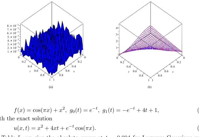
Figure 2. (a) Absolute errors of the solution, (b) Analytical (line) and estimated (point) solutions with dx=dt= 0.0833 andε= 0.9 for Example 2.

f(x) = cos(πx) +x2, g0(t) =e−t, g1(t) =−e−t+ 4t+ 1, (4.5)

(10)

x Method [5] Present method with

uex uhpm M=N=12,ε=0.9 M=N=16,ε=1.3 0.1 0.9429 0.9429 9.8069E–06 5.6883E–08 0.2 0.8340 0.8340 1.0682E–05 1.2380E–07 0.3 0.6675 0.6675 9.9480E–06 9.7971E–08 0.4 0.4646 0.4646 1.2549E–05 5.1661E–08 0.5 0.2520 0.2520 1.3E–06 4.4E–08 0.6 0.0594 0.0594 1.1261E–05 1.6136E–07 0.7 -0.0835 -0.0835 1.0286 E–06 1.2797E–07 0.8 -0.1500 -0.1500 1.0118E–05 5.8276E–08 0.9 -0.1189 -0.1189 8.9131E–06 9.2117E–08

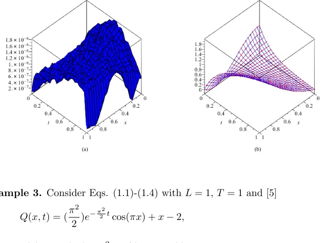
Figure 3. (a) Absolute errors of the solution, (b) Analytical (line) and estimated (point) solutions with dx=dt= 0.0833 andε= 0.9 for Example 3.

Example 3. Consider Eqs. (1.1)-(1.4) withL= 1, T = 1 and [5]

Q(x, t) = (π

2

2 )e

−π2

2 tcos(πx) +x−2, (4.7)

f(x) = cos(πx) +x2, g2(t) =t, g3(t) = 2 +t, (4.8)

u(x, t) =x2+xt+e−π 2

2tcos(πx). (4.9)

(11)

with shape parameterε= 1.3. The absolute errors of our method are compared with the analytical and numerical solutions for homotopy perturbation method (HPM) [5]. The absolute errors of estimated solution, and the exact and estimated solutions are given in Figure 3.

5. Conclusion

A RBF-based numerical method proposed to solve the heat conduction problem with Dirichlet and Neumann boundary conditions. The Laguerre-Gaussians radial basis functions (LG-RBFs) on intervalst∈[0,1] andx∈[0,1] were employed. The method was based upon reducing the system into a set of algebraic equations. The proposed method was tested on several examples given in the literature. The ob-tained results showed that this approach can solve the problem eﬀectively. Moreover, the method is more convenient for implementation in comparison to traditional tech-niques.

Acknowledgements

The authors are very grateful to the referees for carefully reading the paper and for their comments and suggestions which have improved the paper.

References

[1] E. Ashpazzadeh, M. Lakestani, and M. Razzaghi, Cardinal Hermite interpolant multiscal-ing functions for solvmultiscal-ing a parabolic inverse problem, Turkish journal of mathematics. DOI 10.3906/mat-1609-3.

[2] I. Babuska and J. Melenk,The partition of unity method, Int. J. Numer. Methods Eng.,40(4) (1997), 727–758.

[3] A. Cheniguel and A. Ayadi,Solving Non Homogeneous Heat Equation by the Adomian Decom-position Method, Int. J. Numer. Meth. Appl.,4(2010), 89–97.

[4] A. Cheniguel,Numerical Method for Solving Heat Equation with Derivative Boundary Condi-tions, Proceedings of the World Congress on Engineering and Computer Science, San Francisco, USA, October 2011.

[5] A. Cheniguel, Numerical Method for the Heat Equation with Dirichlet and Neumann Condi-tions, Proceedings of the International MultiConference of Engineers and Computer Scientists, Hong Kong, March 2014.

[6] B. Fornberg, T. Dirscol, G. Wright and R. Charles,Observations on the behavior of radial basis function approximations near boundaries, Comput. Math. Appl.,43(2002), 473–490.

[7] R. Franke,A Critical Comparison of Some Methods for Interpolation of Scattered Data, 1979. Thesis (Ph.D.)– Naval Postgraduate School Monterey - California.

[8] R. L. Hardy, Multiquadric equations of topography and other irregular surfaces, J. Geophys. Res.,76(8) (1971), 1905–1915.

[9] J. H. He, A coupling Method of Homotopy Technique for Non Linear Problems, Int. J. Non Linear Mech.,35(1) (2000), 37–43.

[10] J. H. He,Homotopy Perturbation Technique, Comput. Meth. Appl. Mech. Eng.,178(3-4) (1999), 257–262.

[11] E. Kreyszig, Introductory Functional Analysis with Applications, John Wiley & Sons Press, New York, 1978.

[12] C. Micchelli,Interpolation of scattered data: distance matrices and conditionally positive deﬁ-nite functions, Constr. Approx.,2(1) (1986), 11–22.

(12)

[14] A. A. Neves, Analysis of laminated and functionally graded plates and shells by a Uniﬁed Formulation and Collocation with Radial Basis Functions, A thesis submitted for the Doctoral Degree, 2012.

[15] S. A. Sarra,Adaptive radial basis function method for time dependent partial diﬀerential equa-tions, Appl. Numer. Math.,54(2005), 79–94.

[16] H. W. Sun and J. Zhang, A high-order compact boundary value method for solving one-dimensional heat equations, Numer. Methods Partial Diﬀerential Equations.,19(6) (2003), 846– 857.

[17] E. Tohidi and A. Kılı¸cman, An eﬃcient spectral Approximation for solving several types of parabolic PDEs with nonlocal boundary conditions, Math. Probl. Eng.,2014(2014), 6 pages. [18] H. Wendland,Piecewise polynomial, positive deﬁnite and compactly supported radial functions

of minimal degree, Adv. Comput. Math.,4(1) (1995), 389–396.

[19] Z. M. Wu,Radial basis function scattered data interpolation and the meshless method of nu-merical solution of PDEs, Chin. J. Eng. Math.,19(2) (2002), 1–12.

[20] Z. M. Wu and R. Schaback, Local error estimates for radial basis function interpolation of scattered data, IMA J. Numer. Anal.,13(1) (1993), 13–27.

[21] D. Yambangwai and N. Moshkin, Deferred Correction Technique to Construct High-Order Schemes for the Heat Equation with Dirichlet and Neumann Boundary Conditions, Engineering Letters.,21(2) (2013), 61–67.