Max Planck Institute for Demographic Research Konrad-Zuse Str. 1, D-18057 Rostock·GERMANY www.demographic-research.org
DEMOGRAPHIC RESEARCH
VOLUME 21, ARTICLE 5, PAGES 109-134
PUBLISHED 07 AUGUST 2009
http://www.demographic-research.org/Volumes/Vol21/5/ DOI: 10.4054/DemRes.2009.21.5
Research Article
An analysis of life expectancy and economic
production using expectile frontier zones
Sabine K. Schnabel
Paul H.C. Eilers
c
°2009 Sabine K. Schnabel & Paul H.C. Eilers.
2 An overview of previous research 111
2.1 Life expectancy and GDP 112
2.2 Models for frontier estimation 113
2.2.1 Quantile regression 113
2.2.2 Econometric methods for efficiency estimation 113
2.3 Data description 114
3 Least Asymmetrically Weighted Squares Smoothing 116
3.1 LAWS in a nutshell 117
3.2 Extreme observations 119
3.3 Theoretical expectiles 119
3.4 What do we call a frontier? 120
3.5 Individual performance measures 122
4 Data analysis 122
4.1 Expectile estimation for different periods 122
4.2 Performance estimation 123
5 Discussion 127
6 Acknowledgement 130
An analysis of life expectancy and economic production using
expectile frontier zones
Sabine K. Schnabel1
Paul H.C. Eilers2
Abstract
The wealth of a country is assumed to have a strong non-linear influence on the life ex-pectancy of its inhabitants. We follow up on research by Preston and study the relationship with gross domestic product. Smooth curves for the average but also for upper frontiers
are constructed by a combination of least asymmetrically weighted squares andP-splines.
Guidelines are given for optimizing the amount of smoothing and the definition of fron-tiers. The model is applied to a large set of countries in different years. It is also used to estimate life expectancy performance for individual countries and to show how it changed over time.
1corresponding author; Max Planck Institute for Demographic Research, Rostock, Germany and Biometris,
Wageningen University and Research Center, Wageningen, The Netherlands;[email protected]
1. Introduction
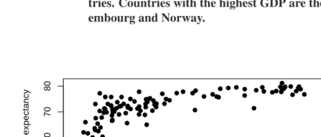
It is well known that life expectancy at birth (e0) is higher in wealthy countries. This
is supported by Figure 1. This association was first investigated by Preston (Preston 1975, 1976). There is a curvilinear relationship between period life expectancy and gross domestic product per capita (GDP). Large scatter is observed around the trend, generally wider at low GDP. A natural question to ask is whether we can estimate a “frontier”,
a curve of the highest attainablee0 against GDP. Such a frontier would be of value to
demographers who study groups of countries. It could also be an important tool for policy makers in individual countries in order to set goals for public health systems.
Figure 1: Average life expectancy versus gross domestic product per capita
in 1990 PPP dollars. Data for the year 2000 including 126 coun-tries. Countries with the highest GDP are the United States, Lux-embourg and Norway.
0 5000 10000 15000 20000 25000 30000
40
50
60
70
80
GDP
Average life expectancy
curve. The principle we use is known as asymmetric least squares or least asymmetrically
weighted squares (LAWS3).
In this paper we will use the word frontier in a soft interpretation, i.e., as a frontier zone that is located in the upper part of the data. Most data points will be located under the estimated curve, but some of the observation might also be found above the curve due to sampling variation and other factors. Therefore, in the following, the use of the word frontier is equivalent to a frontier zone and not used as an absolute boundary.
Smoothing with LAWS is a simple and easily implemented idea. It also poses new and interesting challenges. One is the choice of the optimal amount of smoothing. We show that ideas from mixed model technology can be applied fruitfully for this purpose, leading to an automatic choice of the amount of smoothing. A second problem is the choice of the amount of asymmetry that defines the frontier. We have no statistical answer to that, but we provide a practical rule of thumb.
The relationship between GDP ande0 has been studied extensively. In Section 2.1
we give an overview of the literature. As far as we know, we are the first to propose and apply a general framework for frontier estimation in the context of life expectancy. In other areas, especially for frontier and efficiency estimation in econometrics, other approaches have been used. We give a short overview of them in Section 2.2. The demo-graphic data that motivated our research is presented in detail in Section 2.3. Section 3 presents LAWS and its application to smoothing, including the determination of the opti-mal amount of smoothing. We also discuss the issue of removal of influential data points and outliers. We show how to compute LAWS statistics for theoretical distributions and use it to propose guidelines for setting the amount of asymmetry. Section 4 lays out the extensive application of LAWS to life expectancy data that motivated this research. The proposed method is also useful for other relations and other explanatory variables than the one presented in the example. In the final section 5 we discuss our results, desirable improvements and possible extensions.
2. An overview of previous research
This section offers an overview of previous research. Because of the intended demo-graphic audience we give a presentation of what has been published on the relationship between life expectancy and gross domestic product per capita. We give less space to the literature on quantile regression and models for efficiency estimation.
3A common abbreviation is ALS, but we like to avoid it for two reasons: first, ALS is also commonly used as
2.1 Life expectancy and GDP
Historically the development of life expectancy has been an important topic in population studies. In Bengtsson (2006) a collection of articles on the linear rise in life expectancy and its history and prospects can be found. For our investigations the contribution of (Oeppen 2006) is of special interest. It reviews life expectancy development and related research since 1820. Over decades researchers have hypothesized about the limits to life expectancy. In (Oeppen and Vaupel 2002) the authors review these hypotheses. However, the article’s main finding about the development of life expectancy is that record life expectancy has been increasing linearly over the last 150 years. This measure can be considered a frontier to life expectancy and thus promotes the interest in investigating limits and appropriate methods for their estimation.
In the 1970s the demographer Samuel Preston investigated the influence of economic conditions on life expectancy (Preston 1975, 1976). For the mean curve of this relation-ship he used a logistic model with fixed coefficients. Three waves of data from 1900, 1930 and 1960 were used in this cross-sectional analysis. As a measure of economic perfor-mance Preston used national income per capita as the independent variable to model the mean trend. The logistic model that Preston used to describe the relationship is a restric-tive assumption of the functional form of this relationship. To our knowledge Preston’s work has never been formally extended to measure the frontier but focusses on describing the mean trend, although Easterlin (1996) stated that Preston’s curve could be described as a production frontier of income as input and life expectancy as output.
Preston’s research was reprinted 30 years later (Preston 2007a) and joined by an ex-tensive discussion and rejoinder by the author (Preston 2007b). The contributions in the discussion stress the importance of health interventions on mortality development (Ku-nitz 2007), and the contribution of technical progress to population health (Bloom and Canning 2007), and discuss why the same amount of income can buy progressively more health over time (Wilkinson 2007). Riley (2007) highlights the fact that more research is needed in order to determine factors influencing life expectancy other than income alone and stresses that countries’ mortality histories need more attention.
Deaton (2004) also refers to Preston’s study and fits a non-parametric population-weighted regression function for the mean relationship between per capita GDP and life expectancy for the year 2000.
contri-bution was reprinted in Rodgers (2002) and joined by a discussion including Wilkinson (2002), Porta, Borrell, and Copete (2002), Deaton (2002) and Lynch and Smith (2002).
Others argue that the mean level of income is not as important to life expectancy as how this money is distributed. Wilkinson also contributed to this field of research con-cluding that there is a lack of association between gross national product (GNP) per capita (measured in 1985 US dollars) and life expectancy in developed countries (Wilkinson 1990). He argues that with better comparability of international data in terms of GNP this association needs more research. When instead he uses purchasing power parity adjusted GNP per capita in a later paper (Wilkinson 1992) he finds a weak association between GNP per capita and combined life expectancy for the 23 OECD countries.
Becker, Philipson, and Soares (2003) investigated longevity convergence and also the relationship between income and longevity referring to and confirming Preston’s study using a logarithm function for data from 1965 and 1995. They conclude that there is no convergence in income per capita in this period despite longevity convergence. This is consistent with a shift over time of the cross-sectional relationship. While the described
relationship holds for the mean trend ofe0 and GDP, it has never been tested to model
frontiers.
2.2 Models for frontier estimation
2.2.1 Quantile regression
Quantile regression is a popular tool for the purpose of frontier estimation. It was orig-inally presented by Koenker and Bassett (1978) as a generalization of the linear model. Quantile regression is based on asymmetrically weighting the sum of absolute values of residuals. It estimated the conditional quantile functions of the underlying distribution. In contrast to quantile regression we propose asymmetrically weighting the sum of squared residuals that leads to so called expectiles as introduced by Newey and Powell in 1987. LAWS is based on ordinary least squares modeling and thus shares the properties and the simple concept of this approach.
2.2.2 Econometric methods for efficiency estimation
of Kumbhakar and Lovell (2000) gives a comprehensive overview of SFA. Assuming a certain error distribution, it can be shown that LAWS is equivalent to SFA. This relation-ship can be deduced from Aigner, Amemiya, and Poirier (1976) and Newey and Powell (1987). Both DEA and SFA are used to estimate frontiers of a multiple input-output re-lation to measure the efficiencies of the individual observations. For example, they were used to describe the relationship between healthy life expectancy and health care status of a country in Evans et al. (2001); Hollingsworth and Wildman (2003). In addition to DEA and SFA Kokic et al. (1997) propose M-quantiles to model production frontiers. It can be shown that there is a relationship between expectiles and M-quantiles (Jones 1994). Kokic et al. also describe how to use M-quantiles to measure productive efficiency.
2.3 Data description
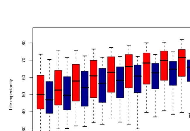
In the analysis in Section 4 we focus on the same variables as Preston and investigate the relationship between life expectancy at birth (average as well as sex-specific) and the logarithm of gross domestic product per capita (logGDPpc) expressed in 1990 purchasing power parity adjusted (PPP) Geary-Khamis dollars. PPP adjustment goes back to Karl Gustav Cassel who developed this concept in the 1920s. The Geary-Khamis method combines the concepts of PPP and average international prices. This technique was first introduced in Geary (1958) and further developed by Khamis (Khamis 1969, 1970, 1972). It is the most widely used method in this field, e.g. by the United Nations, OECD, the statistical office of the European Union and others. For our analysis we use data from 1900 to 2005. The sample size in the waves is varying. Therefore we limit further analysis to years with at least 20 countries in the sample. This is the case for 66 years between 1900 and 2005 (1900, 1910, 1920, 1930, 1940 and every year between 1945 and 2005). Life expectancy data come from a range of sources including the HMD (Human Mortality Database 2007), national statistical offices, the Penn World tables (Heston, Summers, and Aten 2002) and the United Nations. Information on logGDPpc was also gathered from a range of sources that include the above, contributions by Maddison e.g. (Maddison 2001) and data from the Total Economy Database (The Conference Board and Groningen Growth and Development Centre 2006). Some descriptive measures of the data set can be seen in Figure 2. The data includes over 200 countries at different points in time.
Figure 2: Box-plots of life expectancy of women (red) and men (blue) 1950– 2000 in five year intervals. The number of countries available in
each year is given by the sample sizenindicated below each
box-plot.
Year
Life expectancy
103 98 102 102 112 105 104 112 127 125 126
n=
1950 1955 1960 1965 1970 1975 1980 1985 1990 1995 2000
20
30
40
50
60
70
80
Women Men
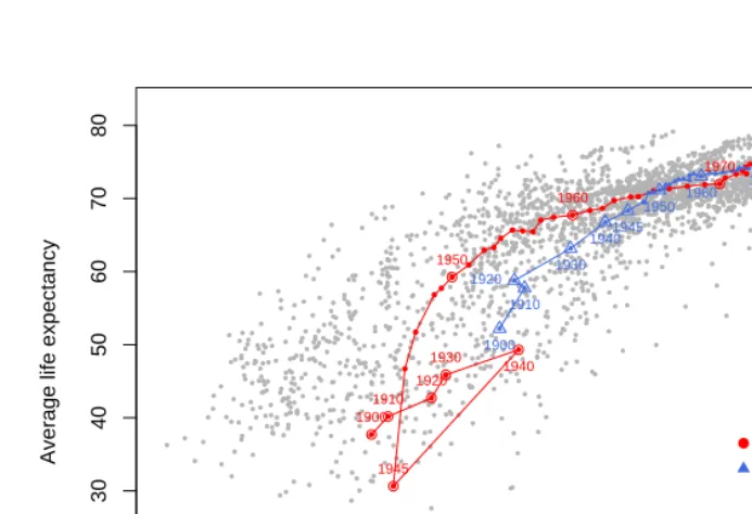
Historically, Japan experienced big gains in this measure after World War II and in-creasing development ever since. Sweden is a country with a long time series of data and it has always been among the countries with the highest life expectancy worldwide.
Figure 3: Pooled data over all years. Development of average life expectancy over time in Japan (red circles) and Sweden (blue triangles).
2.5 3.0 3.5 4.0 4.5
20
30
40
50
60
70
80
logGDPpc
Average life expectancy
1900 1910
1920 1930
1940
1945 1950
1960
1970 1980
1990 2000
2005
1900 1910 1920
1930 19401945
1950
1960 1970 19801990
20002005
Japan Sweden
3. Least Asymmetrically Weighted Squares Smoothing
3.1 LAWS in a nutshell
In ordinary least squares (OLS) estimation one seeks to minimize the sum of squares
SOLS = X
i
(yi−µi)2
whereyiis the response andµiis the estimated value. For example, in linear regression
isµi= ˆβ0+ ˆβ1xiwithβˆthe estimated coefficient vector.
Least asymmetrically weighted squares estimation (LAWS) seeks to minimize the
following objective function for a range of valuesp,0< p <1:
S = X
i
wi(p)(yi−µi(p))2 (1)
with weights
wi(p) = ½
p ifyi> µi(p)
1−p ifyi≤µi(p) (2)
whereyiis the response variable andµi(p)is the estimated value according to a
statisti-cal model. The obtained functionsµ(p)are calledp-expectilesas introduced by Newey
and Powell in 1987. LAWS is a weighted version of ordinary least squares where the weights depend on the sign of the residuals. When estimating an expectile, we fix a value
pbetween 0 and 1. For an upper frontier we may choose e.g. p = 0.98. In the
iter-ative fitting procedure each pointi of the data set is assigned a weightwi(p = 0.98)
according to (2). This means a point located above the estimated curveµ(0.98)receives
a weightwyi>µi(0.98)= 0.98. A data point below or on the estimated curve is assigned
weightwyi≤µi(0.98) = 0.02. OLS estimation is a special case of LAWS forp= 0.5. It
is extremely easy to fit any LAWS model: simply iterate between weighted regression and re-compute the weights. The objective function is convex, so a unique minimum is guaranteed.
For simplicity, we suppress the dependence onpin the following notation.
When implementing a flexible functional form of the expectile, we combine LAWS
withP-splines (Eilers and Marx 1996): µi =
P
jbijaj, whereB = [bij]is the matrix
ofB-spline basis functions andathe coefficient vector. A penalty tunes the smoothness.
Thus we are seeking to minimize the penalized LAWS function:
S∗= (y−Ba)TW(y−Ba) +λkD dak2
The model parameters are computed iteratively according to
ˆ
a = (BTW Bf +P)−1BTW yf
with current weights infW =diag( ˜w)and the penaltyP =λDT
dDd.
To optimize the smoothing parameter λwe can use so called leave-one-out
cross-validation. The idea is to remove each observation (xi,yi) in turn, predict it (µ−i) from
the remaining ones and measure prediction performance by the cross validation score
CV = 1
n
Pn
i=1(yi−µ−i)2. The asymmetric variant includes the weights according to
(2):
ACV = 1
n
X
i
wi(yi−µ−i)2= 1
n
X
i
wi(yi−µi)2
(1−hii)2 ,
where we have used the fact thatyi−µ−i= 1−yi−hµiii with the hat matrixH = (hij)i,j=1,...,n
defined as
H = W12B(BTW B+P)−1BTW12. (3)
We search for the minimumACV for a range of values ofλon a grid (linear forlogλ).
This is done separately for everyp. In theACV we assume that the weight vector is
invariant to single missing observations. Simulation studies show that this assumption
holds for more than99%of the considered cases.
Alternatively, using the formal equivalence between penalized least squares smooth-ing and mixed models (Pawitan 2001; Lee, Nelder, and Pawitan 2006), we have that the
smoothing parameterλ = σ2
τ2, withσ2 the variance of the weighted errors andτ2 the
variance of the contrastsDa. We estimate these variances by
ˆ
σ2= (y−µ)
T
W(y−µ)
n−ED , τˆ
2=kDak 2
ED
wheren is the sample size and ED = trace(H) the effective model dimension. We
iterate between smoothing asymmetrically withλ, estimating variances (and a newλ)
until convergence (inλand ideally also in weights). This is a variant of Schall’s (1991)
method for generalized linear mixed models.
In the application in Section 4 we use optimal smoothing according to Schall’s algo-rithm. This technique gives very similar results to the use of cross-validation criteria, but due to its iterative set-up it is computationally less intensive, particularly with large data sets.
3.2 Extreme observations
In order to improve the quality and robustness of the estimation, outlier detection is com-monly used in regression methods. This can be also done in the model framework pre-sented above. We make use of the hat matrix from the estimation procedure in order to
identify outliers or so-calledextreme observations. For linear regression (Hoaglin and
Welsch 1978) suggested as a rule of thumb those points with
hii>
2ED
n
to qualify for an extreme point, i.e. an influential observation. In our context we use the
hat matrixH of the model as defined in (3) and fornthe respective sample size of the
analyzed wave. We suggest that the points which were commonly classified as extreme
observation for at least 80 of the 99 expectiles with0.01≤p ≤0.99(in increments of
0.01) are excluded from the analysis and the entire set of expectiles re-estimated. In order to further check for extreme observations in the vertical direction we suggest checking
for candidates against the mean curve forp= 0.5. As a rule of thumb, a pointiwill be
classified as an extreme observation in the vertical direction if
|yi−µi(0.5)|>3SD
as a rule of thumb. SD is the empirical standard deviation of the residuals. We propose to remove the detected points to improve the data quality.
With this methodology, we propose a statistical criterion for judging about potential extreme observations and their removal from the data set. However, in any application it might be also useful to exclude other observations from the data under consideration based on particularities of the data, data quality or other arguments.
3.3 Theoretical expectiles
Expectiles can also be computed for theoretical distributions. Assume we have a
proba-bility density functionf(x)with
F(x) =
x Z
−∞
f(u)du and G(x) =
x Z
−∞
uf(u)du.
HereF(x)is the distribution function, i.e. the cumulative density, andG(x)is the partial
seek to minimize (1) with weights according to (2). For a continuous distribution this is equivalent to
min
ep
(1−p)
ep
Z
−∞
(u−ep)2f(u)du+p
∞
Z
ep
(u−ep)2f(u)du.
Minimizing this form leads to
(1−p)
ep
Z
−∞
(u−ep)f(u)du+p
∞
Z
ep
(u−ep)f(u)du= 0.
After some algebra and replacement forF(x)andG(x)we can determine the theoretical
p-expectileepby
ep=(1−p)G(ep) +p(m−G(ep))
(1−p)F(ep) +p(1−F(ep))
withmthe mean of the underlying distributionF andG(∞) =m. Solving forp, with
z=ep, we get
p= G(z)−zF(z)
2(G(z)−zF(z)) + (z−m). (4)
This relationship follows from (Newey and Powell 1987; Jones 1994). According to Theorem 1 in the latter article, expectiles shift and scale like expected values with changes
in meanmand standard deviationσoff(x|m, σ).
In order to determine the theoretical expectiles of a distribution, we choose a sensible
grid forzand compute the corresponding vector ofps by numerical inversion.
3.4 What do we call a frontier?
In the framework of expectile estimation it is up to the user what to choose as an upper
frontier in terms of parameterp.
As seen above it is possible to estimate the expectile at almost anyp∈(0,1). In the
context of frontier estimation we are looking to identify a suitable frontier for the given
relationship. Therefore we have to decide on an appropriate value forp. We may use a
common distribution as the reference distribution, e.g. the standard normal distribution.
According to (4) in the standard normal case we havepas
p = φ(z) +zΦ(z)
2φ(z) + 2zΦ(z)−z
withφ,Φthe respective density and distribution function of the standard normal
distri-butionN(0,1). Choosingzequidistant in[−3,3]covers values ofpin almost the entire
range from 0 to 1.
It is up to the user to decide which value ofpto choose for a frontier to be estimated.
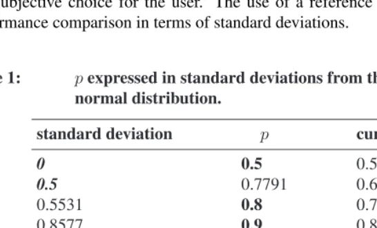
With the help of Table 1 the user can get a better insight into what a certain value forp
would be in terms of the normal distribution as a reference. In our opinion 2 standard
normal deviations (orp= 0.9958) might be a good choice for a frontier. However, this
is a subjective choice for the user. The use of a reference distribution also allows for performance comparison in terms of standard deviations.
Table 1: pexpressed in standard deviations from the mean of a standard
normal distribution.
standard deviation p cumulative density
0 0.5 0.5
0.5 0.7791 0.6915
0.5531 0.8 0.7099
0.8577 0.9 0.8045
1 0.9286 0.8413
1.1383 0.95 0.8725
1.4749 0.98 0.9299
1.5 0.9812 0.9332
1.7154 0.99 0.9569
2 0.9958 0.9772
2.5 0.9992 0.9938
Note that the reference distribution is being used here only as a guide for selecting
values ofp. It is possible and useful to compare the empirical expectiles with theoretical
expectiles of the reference distribution, but we do not pursue this approach here.
3.5 Individual performance measures
Kokic et al. (1997) propose M-quantiles to model production frontiers and to measure productive efficiency. According to Jones (1994) there is a relationship between expectiles and M-quantiles. From previous applications in this area (see Hollingsworth and Wildman 2003) as well as from the theoretical connections we suggest efficiency analysis in the context of LAWS. As a variant of the definition suggested in Kokic et al. (1997) we assign
as value for the so calledperformancethe valuepof the closestp-expectile (in terms of
absolute distance):
performance(xi) = min
p arg|yi−µi(p)|. (5)
In order to receive a wide range of possible performance values in a sample we
es-timate a dense grid ofp-expectiles. In the analysis in Section 4.2 we applied this
per-formance measure to data on life expectancy and GDP in an investigation of sex-specific reactions to improvement in the economic performance of a single country, and include as well comparisons between countries.
This relative performance measure is an approximation on the grid of usedp’s. It will
be possible to develop a technique that helps us to find the exactp-expectile for a given
data point.
4. Data analysis
4.1 Expectile estimation for different periods
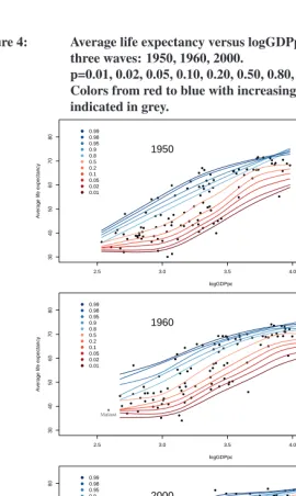
In this section we present results from the analysis of selected waves. We chose the years 1950, 1960 and 2000 (with sample sizes of 101, 99 and 126 countries respectively). After
estimating a set of expectiles – namely 99 curves with0.01≤p≤0.99– we proceeded
low life expectancy for the level of nominal wealth. After removing these observations the estimated expectiles improved. This can be seen in Figure 5 where we present the estimated set of expectiles for 1950 before and after removing extreme observations. It has also been pointed out in (Yee 2008) that expectiles are more susceptible to outliers than the more robust quantile estimation. This supports our approach to combine outlier detection with estimating expectiles.
We chose the years 1950 and 1960 in order to see potentiale0 increases associated
with increases in GDP following the post-war economic boom. Range, variance and composition of the three data sets differ. This leads to different characteristics in the estimated curves. The spread of the estimated expectiles is smaller in 1960 than in 1950.
However, the mean distance betweene0.9ande0.1is about the same. The smaller spread
of expectiles is seen again in 2000. The expectiles confirm the hypothesis of longevity convergence by Becker, Philipson, and Soares (2003) and are in line with their statement of no obvious convergence in GDP, as in the three years under consideration, the standard deviation for GDP is largest in 2000.
4.2 Performance estimation
While in Figure 3 we plotted the development of life expectancy over time of individual countries in a purely descriptive way, in the following we present plots that can be used to illustrate the performance of individual countries, as introduced in Section 3.5. Estimated frontiers and therefore also performance values depend on the composition of the sample in the respective waves. As mentioned above, data on 200 countries were available at different points in time. However, the maximum sample size in the analysis below is 127
countries. Only complete observations in bothe0and GDP can be used. The
Figure 4: Average life expectancy versus logGDPpc. Selected expectiles for three waves: 1950, 1960, 2000.
p=0.01, 0.02, 0.05, 0.10, 0.20, 0.50, 0.80, 0.90, 0.95, 0.98, 0.99.
Colors from red to blue with increasingp. Extreme observations
indicated in grey.
2.5 3.0 3.5 4.0 4.5
30 40 50 60 70 80 logGDPpc
Average life expectancy UAE Kuwait Qatar 1950 0.99 0.98 0.95 0.9 0.8 0.5 0.2 0.1 0.05 0.02 0.01
2.5 3.0 3.5 4.0 4.5
30 40 50 60 70 80 logGDPpc
Average life expectancy
UAE Malawi Qatar 1960 0.99 0.98 0.95 0.9 0.8 0.5 0.2 0.1 0.05 0.02 0.01
2.5 3.0 3.5 4.0 4.5
30 40 50 60 70 80 logGDPpc
Average life expectancy
Figure 5: Data for 1950. Left panel: estimated curves for all data; right panel: re-estimated curves after removing three extreme obser-vations (grey triangles).
2.5 3.0 3.5 4.0 4.5
30
40
50
60
70
logGDPpc
Average life expectancy
0.99 0.98 0.95 0.9 0.8 0.5 0.2 0.1 0.05 0.02 0.01
2.5 3.0 3.5 4.0 4.5
30
40
50
60
70
logGDPpc
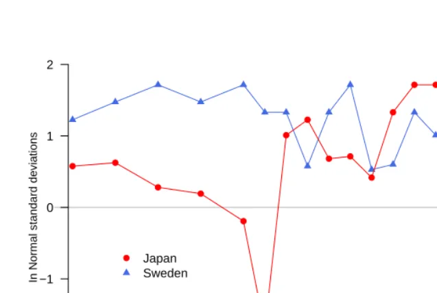
In Figure 6 we plot the relative performance values according to (5) for Sweden and Japan in 1900-2005. As already seen in Figure 3, Japan has a mixed mortality history. This is also true for its relative performance, as its values stretch the entire range between
0.01 and 0.99. The median performance for the displayed years isp = 0.86; in about
30% of the displayed years Japan is closest to the highest estimated frontier curve (with
p= 0.99). Japan has been in the top group in terms of life expectancy, economic level
and relative performance in the last 25 years. In comparison, Sweden historically always
had a high level of relative performance. The series ofpcovers the range from 0.79 to
0.99. The median performance isp = 0.97 and in more than half of the shown years
relative performancepis at least 0.95. Figure 6 shows the scale for relative performance
pand a scale in standard deviations from the mean of the standard normal distribution as
a reference distribution.
Figure 6: Relative performance of Sweden and Japan (average life ex-pectancy versus logGDPpc) on a scale in standard deviations from
the mean of a standard normal distribution (left) and a scale ofp
(right).
Year
1900 1910 1920 1930 1940 1950 1960 1970 1980 1990 2000 −2
−1 0 1 2
0.01 0.02 0.05 0.1 0.2 0.5 0.8 0.9 0.95 0.98 0.99
Performance p
In Normal standard deviations
Japan Sweden
In Figure 7 we depict sex-specific relative performance for four European countries: France, Finland, Germany and the Netherlands.
gap in relative performance is also persistent over time. Germany is the third country in this example. We notice that both sexes are very similar in terms of relative performance, with the level increasing in recent years. The Netherlands is an example of a country with a rapid decline in relative performance over the last 30 years, with the exception of the most recent period. This is especially pronounced for females.
Figure 8 on page 129 depicts the case of Denmark. We present the relative perfor-mance of males and females in the lowest graph. The other two graphs show the life ex-pectancy of Danish males and females along with the estimated expectiles at Denmark’s value of GDP for the respective year. The set of three graphs helps to relate the relative
performance values to the absolute level ofe0and gives a good impression of the spread
in expectiles. The gender gap in life expectancy in Denmark widened considerably from 1950 to 1980, increasing from 3 to a peak of more than 6.5 years. This is followed by a decline to a level of less than 5 years. Females also seem to have systematically lower rel-ative performance values and show a drop in performance during and beyond the period where the gap between female and male life expectancy widened. The causes of stagnat-ing Danish life expectancy, particularly for females, have been explored in (Fiig Jarner, Masotti Kryger, and Dengsøe 2008).
5. Discussion
We developed and applied a new statistical framework to model the relationship between GDP and life expectancy. The core idea is to use least asymmetrically weighted squares (LAWS) to explore not only the central tendency but also extreme regions of the condi-tional distribution. LAWS leads to a very simple iterative estimation algorithm; it is easily
combined withP-splines (B-splines with a discrete roughness penalty) to model trends
and frontiers. By borrowing ideas from mixed models, the weight of the penalty can be optimized straightforwardly. The result is a powerful asymmetric smoother. We compared it to quantile smoothing splines and observed our smoother to be superior (Schnabel and Eilers 2009b).
The smoother was applied to large samples of countries, at different points in recent history. Not only did we compute trends and frontier curves, we also computed perfor-mance measures, a kind of “relative LAWS ranking” to quantify how well each country did over time. We present time series for a number of countries.
Figure 7: Comparison between female and male relative performance for four countries: a scale in standard deviations from the mean in a standard normal distribution (left) and a scale of relative
perfor-mancep(right).
1900 1920 1940 1960 1980 2000
−2 −1.5 −1 0 1 1.5 2 0.01 0.05 0.2 0.5 0.8 0.9 0.98 France
In Normal standard deviations Females Males
Germany
1900 1920 1940 1960 1980 2000
−2 −1.5 −1 0 1 1.5 2 0.01 0.05 0.2 0.5 0.8 0.9 0.98 Performance p Females Males Finland
1900 1920 1940 1960 1980 2000
−2 −1.5 −1 0 1 1.5 2 0.01 0.05 0.2 0.5 0.8 0.9 0.98
In Normal standard deviations Females Males
Netherlands
1900 1920 1940 1960 1980 2000
Figure 8: Relative performance of Danish males and females (lowest panel). For comparison, estimated expectiles at the respective GDP indi-cated in the top panels.
1900 1910 1920 1930 1940 1950 1960 1970 1980 1990 2000 40 50 60 70 80 Life expectancy Males 0.99 0.98 0.95 0.9 0.8 0.5 0.2 0.1 0.05 0.02 0.01
1900 1910 1920 1930 1940 1950 1960 1970 1980 1990 2000 40 50 60 70 80 Life expectancy Females 0.99 0.98 0.95 0.9 0.8 0.5 0.2 0.1 0.05 0.02 0.01
1900 1910 1920 1930 1940 1950 1960 1970 1980 1990 2000 −2 −1 0 1 2 0.01 0.02 0.05 0.1 0.2 0.5 0.8 0.9 0.95 0.98 0.99 Performance p
In Normal standard deviations
What is a frontier? We believe it is a matter of convention, comparable to choosing a 95th or 98th percentile. The LAWS equivalent of quantiles is expectiles. Unfortunately, statisticians and applied scientists as yet have little “feel” for expectiles. We show how to compute expectiles for theoretical distributions and use the results to relate expectiles to
familiarz-scores from the standard normal distribution.
We are convinced that our asymmetric smoother is a valuable tool for demographers and policy makers, because it allows one to visualize and quantify life expectancy
(per-formance). The computations are fast. Our software is written for theRsystem (R
Devel-opment Core Team 2008) and we will be happy to share it.
A serious problem remains in quantile estimation as well as in expectile estimation: the curves can cross. Theoretically this is impossible, but due to sampling variation it is common in practice. Because the LAWS curves are computed in isolation (for each
different value of the asymmetry parameterp), neighboring curves are not taken into
account in the estimation procedure, and cross-overs can occur. In the literature one can find several proposals for creating non-crossing (smooth) quantile curves. In principle these apply to LAWS too. Our experiments indicate that a bilinear or “bundle” model
is a promising alternative: µ(x, p) =a(x)g(p) +b(x), whereµ(x, p)is thep-expectile
curve,b(x)is a trend,g(p)an asymmetry function anda(x)represents the local width of
the expectile bundle. Further details and first results can be found in Schnabel and Eilers (2009a).
6. Acknowledgement
References
Aigner, D.J., Amemiya, T., and Poirier, D.J. (1976). On the estimation of production frontiers: maximum likelihood estimation of the parameters of a discontinuous density
function.International Economic Review17(2): 377–396.doi:10.2307/2525708.
Becker, G.S., Philipson, T.J., and Soares, R.R. (2003). The quantity and quality of life and the evolution of world inequality. National Bureau of Economic Research. (NBER Working Paper Series 9765).
Bengtsson, T. (2006). Perspectives on Mortality forecasting - III. The linear rise in life
expectancy: history and prospects. No. 3 in Social Insurance Studies. Swedish National Social Insurance Agency.
Bloom, D.E. and Canning, D. (2007). Commentary: The Preston Curve 30 years
on: still sparking fires. International Journal of Epidemiology 36(3): 498–499.
doi:10.1093/ije/dym079.
Charnes, A., Cooper, W.W., and Rhodes, E. (1978). Measuring the efficiency of decision
units. European Journal of Operational Research2(6): 429–444.
doi:10.1016/0377-2217(78)90138-8.
Deaton, A. (2002). Commentary: The convoluted story of international studies of
inequality and health. International Journal of Epidemiology 31(3): 546–549.
doi:10.1093/ije/31.3.546.
Deaton, A. (2004). Health in an age of globalization. In: C. Graham and S.M. Collins
(eds.)Brookings Trade Forum 2004 : Globalization, Poverty, and Inequality. Brookings
Institution Press: chap. Globalization and inequality: 83–130.
Easterlin, R.A. (1996).Growth triumphant: the twenty-first century in historical
perspec-tive. The University of Michigan Press.
Eilers, P.H.C. and Marx, B.D. (1996). Flexible smoothing with B-splines and penalties.
Statistical Sciences11(2): 89–121.doi:10.1214/ss/1038425655.
Evans, D.B., Tandon, A., Murray, C.J.L., and Lauer, J.A. (2001). Comparative efficiency
of national health systems: cross national econometric analysis.British Medical
Jour-nal323: 307–310.doi:10.1136/bmj.323.7308.307.
Fiig Jarner, S., Masotti Kryger, E., and Dengsøe, C. (2008). The evolution of death
rates and life expectancy in Denmark. Scandinavian Actuarial Journal 2: 147–173.
doi:10.1080/03461230802079193.
between countries. Journal of the Royal Statistical Society: Series A121(1): 97–99.
doi:10.2307/2342991.
Heston, A., Summers, R., and Aten, B. (2002). Penn World Table Version 6.1. Center for International Comparisons at the University of Pennsylvania (CICUP). (Database).
Hoaglin, D.C. and Welsch, R.E. (1978). The hat matrix in regression and ANOVA. The
American Statistician32(1): 17–22. doi:10.2307/2683469.
Hollingsworth, B. and Wildman, J. (2003). The efficiency of health
produc-tion: re-estimating the WHO panel data using parametric and non-parametric
ap-proaches to provide additional information. Health Economics 12(6): 493–504.
doi:10.1002/hec.751.
Human Mortality Database (2007). [electronic resource]. University of California, Berke-ley (USA) ; Max-Planck-Institut für demografische Forschung, Rostock (Germany). http://www.mortality.org or http://www.humanmortality.de.
Jones, M.C. (1994). Expectiles and M-quantiles are quantiles. Statistics & Probability
Letters20(2): 149–153.doi:10.1016/0167-7152(94)90031-0.
Khamis, S.H. (1969). Neoteric index numbers. Calcutta: Indian Statistical Institute. (Technical report).
Khamis, S.H. (1970). Properties and conditions for the existence of a new type of index
numbers.Sankhya: The Indian Journal of Statistics: Series B32: 81–98.
Khamis, S.H. (1972). A new system of index numbers for national and
interna-tional purposes. Journal of the Royal Statistical Society: Series A 135(1): 96–121.
doi:10.2307/2345041.
Koenker, R. and Bassett, G.W. (1978). Regression quantiles.Econometrica46(1): 33–50.
Kokic, P., Chambers, R., Breckling, J., and Beare, S. (1997). A measure of
pro-duction performance. Journal of Business & Economic Statistics 15(4): 445–451.
doi:10.2307/1392490.
Kumbhakar, S.C. and Lovell, C. (2000). Stochastic Frontier Analysis. Cambridge
Uni-versity Press.
Kunitz, S.J. (2007). Commentary: Samuel Preston’s "The changing relation between
mortality and level of economic development".International Journal of Epidemiology
36(3): 491–492.doi:10.1093/ije/dym076.
Lee, Y., Nelder, J.A., and Pawitan, Y. (2006). Generalized linear models with random
Lynch, J. and Smith, G.D. (2002). Commentary: Income inequality and health:
The end of the story? International Journal of Epidemiology 31: 549–551.
doi:10.1093/ije/31.3.549.
Maddison, A. (1995). Monitoring the world economy 1820-1992. OECD Development
Center.
Maddison, A. (2001).The world economy: a millennial perspective. OECD Development
Center.
Newey, W.K. and Powell, J.L. (1987). Asymmetric least squares estimation and testing.
Econometrica55(4): 819–847.doi:10.2307/1911031.
Oeppen, J. (2006). Life expectancy convergence among nations since 1820:
separat-ing the effects of technology and income. In: T. Bengtsson (ed.) Perspectives on
mortality forecasting - III. The linear rise in life expectancy: history and prospects. Försäkringskassan, Swedish Social Insurance Agency: 55–82.
Oeppen, J. and Vaupel, J.W. (2002). Broken limits to life expectancy.Science296(5570):
1029–1031.doi:10.1126/science.1069675.
Pawitan, Y. (2001). In All Likelihood: Statistical modelling and inference using
likeli-hood. Oxford University Press.
Porta, M., Borrell, C., and Copete, J.L. (2002). Commentary: Theory in the fabric of
evidence on the health effects of inequalities in income distribution. International
Journal of Epidemiology31(3): 543–546.doi:10.1093/ije/31.3.543.
Preston, S.H. (1975). The Changing Relation between Mortality and Level of Economic
Development.Population Studies29(2): 231–248. Reprinted in the International
Jour-nal of Epidemiology Vol. 36, pp.484-490, 2007.
Preston, S.H. (1976). Mortality patterns in national populations. With Special Reference
to Recorded Causes of Death. Academic Press.
Preston, S.H. (2007a). The Changing Relation between Mortality and Level of
Eco-nomic Development - Reprint.International Journal of Epidemiology36(3): 484–490.
doi:10.1093/ije/dym075.
Preston, S.H. (2007b). Response: On "The changing relation between mortality and level
of economic development". International Journal of Epidemiology36: 502–503.
Riley, J.C. (2007). Commentary: Missed opportunities. International Journal of Epi-demiology36(3): 494–495. doi:10.1093/ije/dym078.
Rodgers, G.B. (1979). Income and inequality as determinants of mortality:
an international cross-section analysis. Population Studies 33(2): 343–351.
doi:10.2307/2173539.
Rodgers, G.B. (2002). Income and inequality as determinants of mortality: an
inter-national cross-section analysis (reprint). International Journal of Epidemiology 31:
533–538.
Schall, R. (1991). Estimation in Generalized Linear Models with random effects.
Biometrika78(4): 719–727.doi:10.1093/biomet/78.4.719.
Schnabel, S.K. and Eilers, P.H.C. (2009a). Non-crossing smooth expectile curves. In: J.G.
Booth (ed.)Proceedings of the 24th International Workshop on Statistical Modellung
in Ithaca. Cornell University.
Schnabel, S.K. and Eilers, P.H.C. (2009b). Optimal expectile smoothing. In press at
Computational Statistics and Data Analysis.doi:10.1016/j.csda.2009.05.002.
The Conference Board and Groningen Growth and Development Centre (2006). Total Economy Database. [electronic resource]. Http://www.ggdc.net.
Wilkinson, R.G. (1992). Income distribution and life expectancy.British Medical Journal
304: 165–168.doi:10.1136/bmj.304.6820.165.
Wilkinson, R. (2002). Commentary: Liberty, fraternity, equality. International Journal
of Epidemiology31(3): 538–543. doi:10.1093/ije/31.3.538.
Wilkinson, R.G. (1990). Income distribution and mortality: a ’natural’ experiment.
Soci-ology of Health & Illness12(4): 391–412. doi:10.1111/j.1467-9566.1990.tb00079.x.
Wilkinson, R.G. (2007). Commentary: The changing relation between
mor-tality and income. International Journal of Epidemiology 36(3): 492–494.
doi:10.1093/ije/dym077.
Yee, T.W. (2008). vgamfamily functions for quantile regression. [electronic resource].