Vol. 10, No. 2, 2015, 247-254
ISSN: 2279-087X (P), 2279-0888(online) Published on 17 November 2015
www.researchmathsci.org
247
Annals of
Strong Circuit Matrix and Strong Path Matrix
of a Semigraph
Prabhakar R. Hampiholi1 and Jotiba P. Kitturkar2
1
Department of Master of Computer Science, Gogate Institute of Technology Belgaum, Karnataka, India. E-mail: [email protected]
2
Department of Mathematics, Maratha Mandal Engineering College Belgaum, Karnataka, India. E-mail: [email protected]
Corresponding author
Received 13 October 2015; accepted 2 November 2015
Abstract. In this paper the strong circuit matrix and strong path matrix of semigraphs are defined and their relation with partial edge incidence matrix are obtained. The results of circuit matrix and path matrix of simple graph are generalized in this paper.
Keywords: Strong circuit matrix of semigraph; Path matrix of semigraph AMS Mathematics Subject Classification (2010): 05C50
1. Introduction
The notion of a Semigraph is a new concept introduced by Sampatkumar [5], generalizing the concept of a graph. Semigraph resembles graph when drawn on a plane and every concept/results in graph can be easily generalized yielding a rich variety of corresponding results. Road networks, projective geometry, Steiner’s triple systems are the some examples of semigraphs. Many authors [1,2,3,9,10] have studied properties of semigraphs.
Representation of any discrete structure in matrix form is important for the applications in electrical network analysis, operation research and computer science. Many authors [2,7,12,13] have studied the properties graph, semigraph and fuzzy graph by using their associated matrices. The author [7] defined partial edge incidence matrix of semigraph and author [2] defined the adjacency matrix of semigraph. In this paper strong circuit matrix and strong path matrix of semigraph are defined. The results of circuit matrix and path matrix of graph [4,6] are generalized in this paper.
2. Preliminaries
Definition 2.1. [5] A semigraph G is an ordered pair (V; X) where V is a non-empty set,
whose elements are called vertices of G and a set X is a set of n - tuples, called edges of G, of distinct vertices, for various n≥2, with the following conditions :
SG1: Any two edges have at most one element in common.
SG2: Two edges (u1; u2 ; . . . un) and (v1; v2; . . . ; vm) are considered to be equal if and only if
248
ii) either ui = vi or ui = vn-i+1 for i = 1, 2, 3, . . n
Thus the edge (u1; u2; . . . . un) is the same as the edge (un; un-1; . . . u1).
Let G = (V; X) be semigraph and E = (v1; v2; . . . ; vn-1; vn) is an edge of G. Then the vertices v1 and vn are called the end vertices, represented by thick dots, the vertices v2; . . . . ; vn-1 are called the middle vertices or m-vertices, represented by small hollow circles. A vertex v in G which appears as end vertex of one edge and middle vertex of the other edge is known as the middle-cum-end (m, e) vertex represented by a small tangent to the hollow circle of middle vertex.
Example 2.2. Let G = (V; X) be a semigraph (Figure 1) , where V = (v0; v1; v2; v3; v4 ,v5; v6; v7; v8) and X = ((v0; v1; v2); (v1; v3; v4); (v4; v5); (v5; v6; v7); (v2; v7; v8)) In G, v0; v2; v4; v5; v8 are end vertices, v3 and v6 are middle vertices, v1 and v7 are middle-cum-end vertices.
Figure 1: Semigraph G
Definition 2.3. [5] A subedge of an edge E = (v1; v2; . . . vn) is a k-tuple E’ =(vi1 ; vi2 ; . . . vik ) where 1 ≤ i1 < i2 < . . < ik ≤ n or 1 ≤ ik < i(k+1) < :: < il ≤ n.
Definition 2.4. [5] A partial edge of E = (v1; v2; . . . vn) is a (j - i + 1)-tuple E’(vi; vj) = (vi; vi+1; . . . vj ), where 1≤ i ≤ n.
Definition 2.5. [5] fs-edge is an edge which is either a full edge or a subedge and fp-edge
is an edge which is either a full edge or a partial edge.
Definition 2.6. [1] Let E = (v1; v2; . . . vn) be an edge of a semigraph G. Two subedges Sj = (vj1; vj2 ; . . . vjl ) where 1 ≤ j1 < j2 < . . . < jl ≤ n and Sk = (vk1; vk2 ; . . . ; vkm ) where 1< k1 < . . . < km ≤ n of E are said to be consecutive subedges if vjl = vk1.
Two partial edges Pj = (vj ; vj+1; vj+2 ; . . . vj+l ) and Pk = (vk ; vk+1; . . . vk+m ) of E are said to be consecutive partial edges if vj+l = vk+m
An edge E = (v1; v2; . . . vn) has n - 1 partial edges of cardinality two namely P1 = (v1;v2); P2 = (v2 ; v3); . . Pn-1 = (vn-1; vn) such that Pi and Pi+1 are consecutive partial edges for i = 1; 2; . . . n - 2.
249
Definition 2.7. [5] A walk in a semigraph G is an alternating sequence of vertices and
fs-edges v0E1v2E2 . . . vn-1Envn beginning and ending with vertices, such that vi-1 and vi are the end vertices of the fs-edge Ei, 1 ≤ i ≤ n.
A v0 - vn walk is a trail if any two fs-edges in it are disjoint. Note that in a trail vertices may be repeated.
A v0 - vn path is a v0 - vn trail in which all the vertices are distinct. A cycle is a closed path.
A v0 - vn path is an s-path (or a strong path) if all its fs-edges are fp-edges. Otherwise, it is a w-path (or a weak path). Similarly, we define an s-cycle and a w-cycle.
In Figure 1, v0; v2; v1; v4; v5; v6; v7 is w-path, v0; v1; v3; v4; v5; v6; v7 is s-path, v0; v2; v1; v4; v5; v6; v7; v2; v0 is w-cycle and v1; v3; v4; v5; v6; v7; v2; v1 is s-cycle.
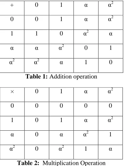
Definition 2.8. [8,11,14] Galois Field of prime power GF(22) is the field of polynomials of degree less than 2 over GF(2) modulo (α2 + α + 1) contains four elements 0; 1; α; α2 = α + 1 where α is a root of the polynomial x2+x+1 ( with coefficients in GF(2) ). The addition and multiplication operation on GF(22) are as shown in the Table 1 and Table 2.
+ 0 1 α α2
0 0 1 α α2
1 1 0 α2 α
α α α2 0 1
α2 α2 α 1 0
Table 1: Addition operation
× 0 1 α α2
0 0 0 0 0
1 0 1 α α2
α 0 α α2 1
α2 0 α2 1 α
Table 2: Multiplication Operation
Definition 2.9. [7] The partial edge incidence matrix B of a semigraph G is a matrix of
order n×m, where n is number of vertices and m is number of consecutive partial edges Pi of cardinality 2 of semigraph G, is defined as
250
= α2, if mm – partial edge Pj is incident on middle vertex vi = 0, otherwise
Figure2: Semigraph G
Example 2.10. For the semigraph G (Figure 2), the partial edge incidence matrix B(G) is
B(G)= 0 1 1 0 0 0 0 0 0 0 0 0 0 0 0 0 0 0 0 0 0 0 0 1 0 0 0 0 0 0 0 0 0 0 0 0 0 0 0 0 0 0 0 1 1 0 0 0 0 0 0 0 0 1 1 0 0 0 0 0 0 1 2 2 2 2 2 2
α
α
α
α
α
α
α
α
α
α
3. Main results
Now we define the strong circuit matrix of semigraph.
Definition 3.1. The strong circuit matrix C = [cij ] of a semigraph G is a matrix of order q×m , where q is number of strong circuit of semigraph G and m is number of consecutive partial edges Pi of cardinality 2 of semigraph G, is defined as
cij = 1, if ith circuit include e-partial edge Pj; = α, if ith circuit include mm-partial edge Pj ; = α2, if ith circuit include me-partial edge Pj ; = 0, otherwise
P9
1
2
3
4 5 7
1
82
P1 P4 P3 P2P6 P7
P8
6
251
The above definition is illustrated in Example 3.2
Example 3.2. For the semigraph G (Figure 2), the strong circuits are
C1 = (P1; P2; P3; P4; P9) , C2 = (P5; P6; P7; P8; P9) and C3 = (P1; P2; P3; P4; P5; P6; P7; P8; P9)
The corresponding strong circuit matrix is
C(G) =
0 1
1 1 0
0 0 0
1 0 0 0 0
2 2
2 2
2 2
2 2
α
α
α
α
α
α
α
α
α
α
α
α
α
α
Remark 3.3. In case of Strong circuit matrix,
• The number of nonzero entries in each row is equal to the number of partial edges of cardinality 2 in the corresponding circuit.
• A column of all zero corresponds to a non circuit edge.
• The permutation of any two columns in a strong circuit matrix corresponds to relabeling of partial edges.
• The permutation of any two rows in a strong circuit matrix corresponds to relabeling of strong circuits.
The following theorem characterizes the strong circuit matrix of a semigraph.
Theorem 3.4. Let C and B be, respectively, the strong circuit matrix and the partial edge
incidence matrix of semigraph (as per the definition 3.1 and the definition 2.9) whose columns are arranged using the same order of partial edges. Then the product BCT or CBT (with respect to GF(22) ) is the matrix containing elements zero or α.
Proof: Consider a vertex v and a strong circuit Ci in the semigraph G. Then either v is in Ci or v is not in Ci . If v is not in Ci , there is no partial edge of cardinality two in Ci that is incident on v. On the other hand if v is in Ci, the number of those partial edges in the circuit Ci that are incident on v is exactly two.
Consider ith row in B and jth row in C. Since partial edges are arranged in the same order, the nonzero entries in the corresponding positions occur only if the particular partial edge is incident on the ith vertex and is also in the jth circuit.
If the ith vertex is not in the jth circuit, then the dot product of the two rows is zero. If the ith vertex is in the jth circuit, then the following ten cases arise.
Case (i) Let ith vertex v is an end vertex and let two partial edges incident on v in circuit Ci are both e-partial edges then the corresponding element in the matrix BCT is (1.1) + (1.1) = 1 + 1 = 0 with respect to GF(22).
Case (ii) Let ith vertex v is an end vertex and let two partial edges incident on v in circuit Ci are both me-partial edges then the corresponding element in the matrix BCT is (1.α2) + (1. α2) = α2 + α2 = 0 with respect to GF(22).
252
corresponding element in the matrix BCT is (1.1) + (1. α2) = 1 + α2 = α with respect to GF(22).
Case (iv) Let ith vertex v is the middle vertex and two partial edges incident on v in circuit Ci are both me-partial edges then the corresponding element in the matrix BCT is (α. α2) + (α.α2) = α3+ α3= 1 + 1 = 0 with respect to GF(22).
Case (v) Let ith vertex v is the middle vertex and two partial edges incident on v in circuit Ci are me-partial edge and mm-partial edge ( represented by α) then the corresponding element in the matrix BCT is (α. α2) + (α2.α) = α3+ α3= 1 + 1 = 0 with respect to GF(22).
Case (vi) Let ith vertex v is the middle vertex and two partial edges incident on v in circuit Ci are both mm -partial edges then the corresponding element in the matrix BCT is (α2.α) + (α2.α) = α3+ α3= 0 with respect to GF(22).
Case (vii) Let ith vertex v is the middle-cum-end vertex and two partial edges incident on v in circuit Ci are me-partial edge and e-partial edge then the corresponding element in the matrix BCT is (α. α2) + (1.1) = α3+ 1 = 1 + 1 = 0 with respect to GF(22).
Case (viii) Let ith vertex v is the middle-cum-end vertex and two partial edges incident on v in circuit Ci are both me-partial edges then the corresponding element in the matrix BCT is (α. α2) + (1. α2) = 1 + α2 = α with respect to GF(22).
Case (ix) Let ith vertex v is the middle-cum-end vertex and two partial edges incident on v in circuit Ci are mm-partial edge and me-partial edge then the corresponding element in the matrix BCT is (α2.α) +(1. α2) = α3+ α2 = 1+ α2 = α with respect to GF(22).
Case (x) Let ith vertex v is the middle-cum-end vertex and two partial edges incident on v in circuit Ci are mm-partial edge and e-partial edge then the corresponding element in the matrix BCT is (α2.α) + (1.1) = α3+ 1 = 1 + 1 = 0 with respect to GF(22).
Therefore, in any case element in the matrix BCT is 0 or α. Similarly, it can be proved for CBT.
Hence the theorem.
Example 3.5. For the semigraph G (Figure 2), let the partial edge incidence matrix B(G)
and strong circuit matrix C(G) are as in Example 2.10 and Example 3.2 then it is clear that
BCT=
α
α
α
α
0
0 0 0
0 0 0
0 0 0
0 0 0
0 0 0
0 0 0
0
Corollary 3.6. Let C and B be, respectively, the strong circuit matrix and the partial edge
253
Now we define the Strong Path Matrix of a Semigraph.
Definition 3.7. A strong path matrix is defined for a specific pair of vertices of a
semigraph, say ( x, y ), and is denoted by P( x, y ). The rows in P corresponds to different paths between vertices x and y, and the columns correspond to the partial edges of G. Path matrix is defined as P( x, y ) =[ pij ] , where
pij = 1, if ith path include e-partial edge Pj ; = α, if ith path include mm-partial edge Pj ; = α2, if ith path include me-partial edge Pj ; = 0, otherwise
Example 3.8. Consider the all different strong paths between vertices 1 and 6 of
semigraph G in Figure 2, L1 = (P9; P6), L2 = (P8; P7; P6) and L3 = (P1; P2; P3; P4; P5). The corresponding 3×9 path matrix is
P =
0 0 0 0
0 1 0
0 0 0 0
1 0 0 0 0
0 0 0
2 2 2
2
α
α
α
α
α
α
α
α
Remark 3.9. In case of strong path matrix,
• A column of all zeros corresponds to an edge that does not lie on any path between x and y.
• A column of all nonzero entries corresponds to an edge that lies in every path between x and y.
• There is no row with all zeros.
The following theorem characterizes the strong path matrix of a semigraph.
Theorem 3.10. If the partial edges of a connected semigraph are arranged in the same
order for columns of partial edge incidence matrix B and the strong path matrix P(x, y), then the product BPT (x; y) = M, (with respect to GF(22) ) where the matrix M has two rows of x and y, are nonzero and the rest of n - 2 rows are zero.
Proof: Proof is similar to Theorem 3.4.
REFERENCES
1. B.Y.Bam and N.S.Bhave, On Some problems of Graph Theory in Semigraphs, Ph.D Thesis, University of Pune.
2. C.M.Deshpande and Y.S.Gaidhani, About adjacency matrix of semigraphs, Intern. Journal of Applied Physics and Mathematics, 2(4) (2012). 250-252
3. D.K.Thakkar and A.A.Prajapati, Vertex covering and independence in semigraph, Annals of Pure and Applied Mathematics, 4(2) (2013) 172-181.
4. D.Narsingh, Graph Theory with Applications to Engineering and Computer Science, New Delhi: Prentice Hall of India Private Limited, (2000).
5. E.Sampathkumar, Semigraphs and their application, Technical Report [DST/MS/22 /94] Department of Science and Technology, Govt. of India, August, 1999.
254
7. P.R.Hampiholi and J.P.Kitturkar, Partial edge incidence matrix of semigraph over GF(22), International Journal of Engineering Research and Technology, 3(9) (2014) 1213-1216.
8. N.Jacobson, Lectures in Abstract Algebra, Volume III Theory of Fields and Galois Theory, D.Van Nostrand Company, Inc. New York (1996).
9. R.Sundareswaran and V.Swaminathan, (m, e)-domination in Semigraphs, Electronic Notes in Discrete Mathematics, 33 (2009) 75–80
10. S.S.Kamath and S.R.Hebbar, Strong and weak domination, full sets and domination balance in semigraph, Electronic Notes in Discrete Mathematics, 15 (2003) 112. 11. S.Lin and D.J.Costello, Error Control Coding, Pearson, 2nd Edition, (2013).
12. S.Meenakshi and S.Lavanya, A survey on energy of graphs, Annals of Pure and Applied Mathematics, 8(2) (2014) 183-191.
13. T.Pathinathan and J.Jesintha Rosline, Matrix representation of double layered fuzzy graph and its properties, Annals of Pure and Applied Mathematics, 8(2) (2014) 51-58.