www.adv-radio-sci.net/14/39/2016/ doi:10.5194/ars-14-39-2016
© Author(s) 2016. CC Attribution 3.0 License.
Extended Kalman Doppler tracking and model determination for
multi-sensor short-range radar
Thomas J. Mittermaier1, Uwe Siart1, Thomas F. Eibert1, and Stefan Bonerz2
1Chair of High-Frequency Engineering, Technical University of Munich, 80290 Munich, Germany 2Ott-Jakob Spanntechnik GmbH, Industriestr. 3–7, 87663 Lengenwang, Germany
Correspondence to:Thomas J. Mittermaier ([email protected])
Received: 14 January 2016 – Revised: 25 April 2016 – Accepted: 29 April 2016 – Published: 28 September 2016
Abstract.A tracking solution for collision avoidance in in-dustrial machine tools based on short-range millimeter-wave radar Doppler observations is presented. At the core of the tracking algorithm there is an Extended Kalman Filter (EKF) that provides dynamic estimation and localization in real-time. The underlying sensor platform consists of several ho-modyne continuous wave (CW) radar modules. Based on In-phase-Quadrature (IQ) processing and down-conversion, they provide only Doppler shift information about the ob-served target. Localization with Doppler shift estimates is a nonlinear problem that needs to be linearized before the lin-ear KF can be applied. The accuracy of state estimation de-pends highly on the introduced linearization errors, the ini-tialization and the models that represent the true physics as well as the stochastic properties.
The important issue of filter consistency is addressed and an initialization procedure based on data fitting and maxi-mum likelihood estimation is suggested. Models for both, measurement and process noise are developed. Tracking re-sults from typical three-dimensional courses of movement at short distances in front of a multi-sensor radar platform are presented.
1 Introduction
The fusion of electronics and mechanics is an ongoing cess, which benefits from by downscaling and reduced pro-duction costs for various kinds of sensor technologies. For monitoring of machine states, all sorts of physical quanti-ties are captured and analyzed. An even more sophisticated task is the prediction of future machine states and of tempo-rary and instantaneous production steps, such as processes in
milling machines. This leads to the notion of collision avoid-ance in automated machine tools in order to prevent damages and downtimes, which cause high maintenance and material costs (Wächter et al., 2014).
For these kinds of industrial machine tools, different ap-proaches of systems for damage reduction are already under investigation, (e.g., Abele et al., 2012). However, for the time being, none of them is able to reliably predict the imminent risk and efficiently avoid collisions by proactive shutdown and deactivation.
In this contribution, the approach of a predictive 24 GHz Doppler surveillance and collision avoidance radar is de-scribed. Extensions and continuations of the fundamental in-vestigations in Wächter et al. (2015), Azodi et al. (2013) and Azodi et al. (2014) are merged. A new signal process-ing stage for nonlinear target trackprocess-ing based on Doppler shift estimates is introduced. It is essentially based on an Extended Kalman Filter (EKF). The algorithm is designed for short-range, single-target tracking. Appropriate process and measurement noise models are derived, test statistics are applied and trajectory estimation is shown. Recently, in-vestigations on solvability, uniqueness of the solution, and the required minimum number of sensors were published by Shames et al. (2013). In the application discussed herein, the solution space for target position and velocity is restricted. Symmetries and ambiguities due to unfavorable sensor place-ment are reduced. Another approach, based on a two-stage filter, was proposed by Battistelli et al. (2013) in order to re-duce the computational costs of a stand-alone particle filter.
underly-ing derived process and noise models, as well as an extensive study on appropriate filter initialization. Additionally, statis-tical tests for filter consistency are introduced. The methods are applied to simulation examples and experimental data de-scribed in Sect. 4. The final conclusion is given in Sect. 5.
2 Problem formulation and Doppler radar model
Within the scope of this work, we consider the following three-dimensional problem: The position of a single target in Cartesian coordinates shall be represented by
p= [x, y, z]T (1)
and may be understood as the mass center of a point scat-terer, which is assumed to be the dominant target compared to all other returns received from a cluttered environment. The observer platform comprisesNsensors with states s(n)= [sx(n), sy(n), sz(n), vx, vy, vz]T, (2) where the sensor positions are known, fixed and related to the origin of the global coordinate system, which lies in the center of the observer platform, see Fig. 1. The velocity vec-tor of the platform isv=vx, vy, vzTand unknown. To get a state vector consisting of full three-dimensional position and velocity, we perform a transformation and assume the observer platform is fixed and the target is moving relative to the platform with just the reversed velocity. Hence, the full target state is
x= [pT,−vT]T= [x, y, z,−vx,−vy,−vz]T. (3) A typical 2-D scenario (z=const) is illustrated in Fig. 1, with two sensors at the positions s(1) and s(2), and a sin-gle moving target (scatterer) at position pwith velocityv. In the following investigation, the radar sensors are assumed to have an isotropic radiation pattern, and they detect a target at distanceks(n)−pkwith Doppler shiftfd(n).
The system equation describes the evolution of the target state with time. The target state at timetkis given by position and velocityx= [pT,vT]T. The kinematic state of the target can be deduced from the previous step tk−1 using the pro-cess matrix Fof a constant velocity (CV) model. Small de-viations from the true trajectory are modeled by zero-mean, white Gaussian noisewk, with corresponding process noise covariance matrix Qk. Then, the following linear discrete-time dynamic model is obtained:
xk=Fxk−1+wk−1, wk∼N(0,Qk). (4) The measurement equation relates the measurements zk to the statexk, where the dimension ofzequals the number of sensors being involved. In mono-static radar systems the ob-served Doppler shift, corrupted by additive zero-mean, white Gaussian measurement noisenk, can be represented by zk=hk(xk)+nk, nk∼N(0,Rk), (5)
Figure 1.Top view (x-y-plane) of the scenario with two sensors at positions(1)ands(2)on a platform with velocityv, illuminating a single target at positionp. The dashed circles represent locations of constant range relative to each sensor. Their intersects are potential position estimates.
whereRk is the measurement noise covariance matrix. The measurement model is given by the nonlinear equation of the Doppler shift observed at thenth sensor
h(n)k (xk)= 2 λ
(s(n)−p k)·vk ks(n)−p
kk
, (6)
where in contrast to Eq. (2), s(n)=hsx(n), sy(n), sz(n) iT
is the sensor position in Cartesian coordinates, for all n=
1, . . ., N.k · kdenotes the Euclidean norm. The radar wave-length λ=c/fc depends on the carrier frequency and the speed of light in the considered medium. Thus,λhas influ-ence on the Doppler sensitivity, which is 160 Hz/(m s−1) in 24 GHz radar systems.
re-Tx/Rx 24 GHz sensors(n)
ui(t)
uq(t)
ADC
fs= 48 kHz A
D
ui(k)
uq(k)
LPF
ˆ
fd(n)
short-time frequency
estimator EKF
xk
Pk
target state
p,v
trajectory estimation
b
x ˆ
fd(N)
ˆ
fd(1)
...
Figure 2.Illustration of the radar system concept and fundamental signal processing blocks for single target multi-sensor tracking. This work is focused on the state estimation algorithm represented by the highlighted part.
spect to the change rate of the state. The ML approach is used only for the initialization procedure to obtain reliable initial states close to the true target state.
3 State estimation via Kalman filtering
For the considered application the EKF is employed. De-spite of the known flaws of the EKF, see e.g. Julier and Uhlmann (2004), first order linearization of the nonlinear Doppler function is assumed to be sufficient, since the sce-narios considered here assume either constant velocity (CV, non-maneuvering) or constant acceleration within a limited range of values. If turning maneuvers and directional changes of motion have to be tracked, UKF is preferred (e.g. Smith, 2008). However, both EKF and UKF, require appropriate ini-tialization of expected values and covariance matrices. Oth-erwise, tracking with these kinds of deterministic filters may lead to poor tracking accuracy or – in case of fatal ambigui-ties – to completely misdirected estimates.
In this section we introduce the adapted EKF algorithm, process and noise models, and give the initialization proce-dure based on maximum likelihood estimation. Furthermore, statistical methods for filter consistency tests are described. 3.1 Tracking filter algorithm
Taylor series expansion is used to linearize the measurement equation around the current target state xk. Second order terms and above are neglected. From Eq. (5) we get
zk=hk(xk)+nk
≈hk(xˆk|k−1)+ ∂
∂xhk(x)(xk− ˆxk|k−1)+nk. (7) This will, from now on, serve as a linear measurement equa-tion to establish the filtering procedure.
The system model consists of the linear equation given by Eq. (4). Now, the standard Kalman Filter equations can be applied for recursive state estimation, see Table 1 for the fil-ter algorithm of an autonomous system (control inputu≡0), with F, Q and R being constant. Noise processes are as-sumed to have zero-mean Gaussian distribution, even though other distributions may be possible and may be tackled by the KF/EKF, which would lead to the best linear estimates.
Table 1.Adapted EKF Algorithm. The initialization is based on MLE, with initial statexˆML, the transition matrixFis linear and
constant, and the measurement equation is linearized.
Initialization
ˆ
x0=E{x0} = ˆxML
P0=E{(x0− ˆx0)(x0− ˆx0)T}
Time Update
ˆ
xk|k−1=Fxk−1|k−1,
Pk|k−1=F Pk−1|k−1FT+Q
Compute Partial Derivative
Hk= ∂ ∂xhk(x)
x= ˆx
k|k−1
Measurement Update
Sk=HkPk|k−1HkT+R Kk=Pk|k−1HkTSk−1
ˆ
xk|k=xk|k−1+Kk zk−hk(xˆk|k−1)
Pk|k=(I−KkHk)Pk|k−1
3.2 Measurement noise model
For experimental investigations low-cost CW radar sensor modules available from RFbeam Microwave GmbH (2014) were used. The signal processing chain consisting of radar sensor, analog-to-digital converter, digital low-pass filter and short-time frequency estimator is given in Fig. 2.
For mutually independent and uncorrelated sensors, the measurement noise covariance matrixRis described by
E{nkn`T} =
0 ifk6=` Rδk` ifk=`,
(8) whereδk`denotes the Kronecker delta. The diagonal matrix Rcan be denoted asR=diag{σ12, σ22, . . ., σN2}.
3.3 Process noise model
The linear drive system of machine tools are capable of fast traverse velocities up to 2 m s−1 and high accelerations up to 10 m s−12. Also, the highly precise position encoder for synchronization of the drive ensures very low deviation from disturbance free motion (e.g. irregular motion and rattling). In this contribution we consider only the non-maneuvering case of constant velocity (CV) with x¨=0, see Bar-Shalom et al. (e.g. 2001, Ch. 6). Small, non-deterministic accelera-tions and deviaaccelera-tions from the ideal rectilinear trajectory are modeled as a zero-mean Gaussian process, see Eq. (4), where
E{wkw`T} =
0 ifk6=`
Qδk` ifk=`. (9)
Measurement and process noise are uncorrelated, as fully de-scribed by E{wkn`T} =0 ∀k, `.
3.4 Filter initialization
For initialization of a tracking filter, usually the expectation value ofx0and the associated covariance matrixP0are used. As prior information about the true meanx0is very limited, a non-Bayesian parameter estimation approach for position and velocity seems to be more appropriate, due to the fact that measurements and the corresponding true target state are very ambiguous and disturbed by noise (Bar-Shalom et al., 2001, p. 91f.). Restrictions due to the given geometry of the observed space in front of the sensor platform and the ve-locity interval from−|vmax|to|vmax|of the drive motor are considered. This leads to a non-convex, but constrained, six-dimensional optimization problem.
The method of maximum likelihood estimation (MLE) is used in consideration of the following circumstances:
– The a-priori knowledge about the true state is uncertain or not sufficient.
– The measurement function (Doppler equation) is highly nonlinear and ambiguous.
– The current target state is a deterministic constant. – The length of the observation intervalkTs does not
in-terfere the constant parameter assumption.
– The measurement noise is a zero-mean Gaussian pro-cess with known covariance matrixR.
The MLE is given by
ˆ
xML=arg max
x p(Z
k|x), (10)
whereZk= {z1, . . .,zk}is the set ofkobservations gathered byN sensors. The likelihood function is given by
p(Zk|x)= 1 p
(2π )nσ2nexp − 1
2σ2 k X
m=1
(zm−h(x))2 !
,
whereh(x)is the Doppler model given by Eq. (6), containing all unknown parameters. Here, the measurement noise is set toR=σ2INfor identical sensor properties.
Next, two extensive simulations are described. Figure 3 depicts the contour plots for MLE for a single measurement (left) and a set of ten sequential measurementsz(right). For illustration, thez- andvz-component were set to zero. In this example the velocity vector was preset and kept constant at v=(−
√
2,
√
2)m s−1 throughout all simulation runs. The frequency estimation uncertainty wasσ=0.1 Hz. The color-bar represents the magnitude of the estimation errorkx− ˆxk. Since the whole geometry is symmetric, including a sym-metric arrangement of ideal, isotropic sensors, the error has symmetric properties in the x-y-plane. This is influenced by the velocity components as well, e.g. if the sign of the vx-component is flipped, the pattern will be mirrored verti-cally. Broad areas with high error levels (top right and bottom left) indicate poor observability and solvability of the equa-tion system due to high similarity of the obtained Doppler shift amongst the sensors. In Fig. 3 (right), significant ac-curacy improvements can be identified if several sequential Doppler estimates were exploited. The sampling interval be-tween each estimate was 1 ms. Improvements can be identi-fied in almost every region. Hence, more accurate initial es-timates can be found by increasing the integration time. Of course, the resulting error characteristic shown in Fig. 3 de-pends on the velocity vectorv. Hence, different velocitiesv result in different regions of poor observability.
A set of different random velocities is investigated next. Figure 4 depicts the absolute errors on position and ve-locity estimates for Monte Carlo (MC) simulations, carried out on a regular grid in space (x∈ [0.3,0.35, . . .,1]m,y∈ [−0.5,−0.45, . . .,0.45,0.5]m,z=0). For every grid point in the z=0-plane, eleven different velocity vectors, each representing an approaching motion, were tested. Addition-ally, the noise level is varied, starting withσf=0.01 Hz up to σf=1 Hz. The resulting errors are below 0.3 m for the posi-tion estimate and below 0.2 m s−1for the velocity estimate. 3.5 Filter consistency
Consistency of a state estimator means that the estimatesxˆ
Figure 3.Error contour plot of a two-dimensional scenario for MLE, exploiting a single Doppler estimate (left) and a set of ten (right) sequential Doppler estimatesZk, with an integration time of 1 ms resp. 10 ms. The velocity vector was preset tov=(−
√
2, √
2)m s−1. A non-coherent uniform linear array (ULA) with five sensors of length 0.4 m serves as observer. The standard deviation of the frequency estimation uncertainty of each sensor was set toσf=0.1 Hz. The colorbar represents the magnitude of the estimation errorkx− ˆxk.
10-4 10-3 10-2 10-1 100
Measurement noise variance 0
0.1 0.2 0.3
M
ag
n
it
u
d
e
of
er
ro
r
(p
os
it
io
n
)
10-4 10-3 10-2 10-1 100
Measurement noise variance 0
0.1 0.2 0.3
M
ag
n
it
u
d
e
of
er
ro
r
(v
el
o
ci
ty
)
Figure 4.Averaged error magnitudes for increasing measurement noise variancesσf2. As shown in Fig. 3, a non-coherent ULA of five sensors is used, and sequential Doppler estimatesZk, with an integration time of 10 ms. For each grid point, the velocity vector was varied according to a set of 11 randomly defined, different approaching movements towards the ULA.
This definition differs from parameter estimation, where con-sistency is an asymptotic property and an infinite set of sam-ples is assumed.
The preferred measure for checking filter consistency in MC simulations is the covariance matrix Pk|k, which is re-lated to the estimate errorexk|k=(xk− ˆxk|k). The normal-ized state estimation error squared (NEES) is defined by the quadratic form
NEES= ex
T k|kP
−1
k|kexk|k. (12)
Asexk|k is Gaussian, the NEES is the sum of the squares of nxindependent zero-mean, unity-variance, Gaussian random variables. The filter is consistent, if the NEES hasχn2 distri-bution withnxdegrees of freedom (Bar-Shalom et al., 2001, Ch. 5.4). For illustration, Fig. 5 shows theχn2-distribution for
n=2,4 and 6. Furthermore, the confidence interval forn=
6 is highlighted. In three-dimensional scenarios, the (e.g.) 95 % confidence interval for NEES can be determined from theχ62distribution as
h
χ62(0.025), χ62(0.975)i=[1.237,14.449].
For observation of a set ofN independent samples, the av-erage NEES can be used as a statistical test for filter consis-tency:
NEESavg= 1 N
N X
k=1
0.25
2 4 6 8 10 12 14 16
x p(x)
n= 2
n= 4
n= 6, (95% interval)
Figure 5.Chi-Square distributions with 2, 4 and 6 degrees of free-dom. For the case ofn=6, the 95 % confidence interval is given by [1.237,14.449] (filled area). For optimized illustration, the axis are scaled appropriately.
NEES is restricted to simulations only, as it requires knowledge of the true statexk. An exploitation of the above quantity is impossible if real processes are observed, without knowledge of the true state. In this case a similar statistic can be evaluated, called the Normalized Innovation Squared: NIS=νTkSk−1νk, νk=zk−hk(xk|k−1). (14) The residual covariance matrix Sk=HkPk|k−1HkT+R is part of the measurement update process, see Table 1. This can be applied in simulations, as well as for measurements. For analyzing a set of N independent samples, the average value is used, which is
NISavg= 1 N
N X
k=1
NISk. (15)
Usage of this quantity has several important benefits, e.g. outliers detection and gating capability, as demonstrated in the next section. In the simulated examples (see Fig. 6) the NIS and the 95 % confidence intervals will be given.
It can be shown that E{χn2} =nand var{χn2} =2n. Hence, the quantities NEES, NIS and the averages have to converge to nx resp.nz, if the filter models are correctly designed. These quantities were used in the following to check initial-ization and the running estimate in the simulations.
4 Simulation results
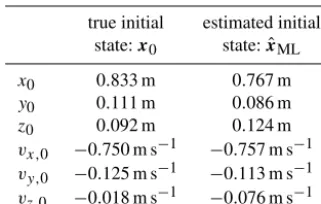
In this section, an illustrative simulation example, performed in Matlab, is described. The scenario is depicted in Fig. 6 (top), with the sensor platform inside the machine tool and six circularly arranged radars on the side front of it. The sen-sor radius is 20 cm. The global origin of the Cartesian coordi-nate system lies in the center of the platform. A single-target is given, moving towards the platform with constant velocity. This represents a typical situation of imminent danger, which has to be handled by a monitoring collision avoidance radar. The initial target state x0 is given in Table 2, together with the initial estimatexˆML obtained from MLE. The ini-tial state covariance matrix is set toP0=0.1I6. These values
-0.2
1 -0.2
0
0.8
z
(m
)
y(m) x(m)
0.6 0.2
0 0.4
0.2 0.2
0
Sensors Init pos. Target trajectory Initialization (MLE) Estimated path
0 200 400 600 800 1000
Sample 0
2 4 6 8 10
Absolute error (cm)
|x−xˆ|
|y−yˆ|
|z−ˆz|
0 200 400 600 800 1000
Sample 0
5 10 15 20 25
NIS
Figure 6.Example of an approaching motion of a point scatterer and tracking results for the applied EKF. The picture on top shows the scenario with six sensors, placed in thex=0-plane, on a ring with radius 20 cm. In the middle, the absolute error of the posi-tion estimate is shown. The bottom picture shows the NIS. The NISavg=5.82≈nzand matches very well with the expectation.
can be derived from the results in Fig. 3. Additionally, the minor diagonal elements are overlaid by low-power additive noise (matrix still symmetric). This leads to improved con-vergence. Furthermore, the process and measurement noise matrices are defined as
R=σf2I6, and (16)
Q=Gσp2GT, (17)
Table 2.Comparison of true and estimated initial state in a simula-tion example. Sampling intervalT =1 ms, integration time 10 ms. The estimation error for positionkp0− ˆpMLkand velocitykv0−
ˆ
vMLkis 0.078 m resp. 0.059 m s−1.
true initial estimated initial state:x0 state:xˆML
x0 0.833 m 0.767 m y0 0.111 m 0.086 m z0 0.092 m 0.124 m vx,0 −0.750 m s−1 −0.757 m s−1 vy,0 −0.125 m s−1 −0.113 m s−1 vz,0 −0.018 m s−1 −0.076 m s−1
has a quite low value. This comes along with low estimation error and the relative high initial covariance matrix. Better overall performance was observed during the MC simula-tions with larger elements in the initial covarianceP0.
Figure 6 (middle) gives an insight into the high track-ing accuracy, with steadily decreastrack-ing estimation error. After 1 s, the final true position isp=(0.083,−0.014,0.073)Tm, which corresponds excellently with the estimated position of
ˆ
p=(0.083,−0.021,0.077)T m. As can be identified from Fig. 6 (middle), the parameterzˆ is the most erroneous one. However, this depends on the sensor configuration. If the sensors are rotated around the x axis, the estimation error
z− ˆz
becomes lower, whereas y− ˆy
is slightly increased. The distancexis a crucial parameter in collision avoidance. It is estimated with sub-centimeter accuracy.
Estimated velocities are not depicted. The estimation prop-erties of the velocities are similar to the coordinates: the es-timation performance forvˆyis better compared tovˆz. This is again due to the sensor arrangement and could be improved by rotating the sensor arrangement. The parametervˆxis esti-mated with very high accuracy.
In Fig. 6 (bottom) the NIS is depicted. This quantity is used for outlier tests, for the gating procedure, and for noise level increasing for the initialization period. Additionally, in Fig. 6 lower and upper bounds of the 95 % confidence inter-vals (χ62-distribution) are given as dashed lines. In this sim-ulation, 95.4 % of all estimates (NIS) are within this accep-tance interval. The time-average NISavghas a value of 5.82, which matches excellently to the expectation ofnz=6.
A further statistical test for correct filter design is the mean-value of the innovationνk, which has to be zero, with associated covariance matrix Sk. In this simulation the ob-tained mean values were in the range−0.04 to 0.08 Hz.
5 Conclusions
This paper presented investigations and results on important issues of Doppler target tracking in short-range scenarios. The utilized Extended Kalman Filter (EKF) was designed
considering the requirements for predictive 24 GHz Doppler radar processing aiming at collision warning and collision avoidance in industrial machine tools. The proposed proce-dure for filter initialization is based on Maximum Likelihood Estimation from several sequential measurements. It deliv-ered reliable initial guesses close to the true target state. In combination with the known restrictions of the considered application, the utilization of a deterministic EKF was inves-tigated. Simulation results confirmed the filter models and showed very high tracking accuracy.
As a next step, we plan to extend the algorithm to handle extended targets with more irregular shapes. In this case we expect that increased Doppler spreading due to multiple scat-tering centers will be observed and a data association prob-lem will arise.
6 Data availability
Datasheet Version 2.0 of K-LC5 Radar Transceiver (RFbeam Microwave GmbH, 2014) is available at http://www.rfbeam.ch/downloads.
This work was supported by the German Research Foundation (DFG) and the Technische Universität München within the funding programme Open Access Publishing.
Edited by: R. Schuhmann
Reviewed by: two anonymous referees
References
Abele, E., Brecher, C., Gsell, S., Hassis, A., and Korff, D.: Steps towards a protection system for machine tool main spindles against crash-caused damages, Prod. Engineer., 6, 631–642, doi:10.1007/s11740-012-0422-6, 2012.
Anderson, B. D. O. and Moore, J. B.: Optimal Filtering, Prentice-Hall, Englewood Cliffs, NJ, USA, 1st Edn., 1979.
Azodi, H., Siart, U., and Eibert, T. F.: A fast three-dimensional deterministic ray tracing coverage simulator for a 24 GHz anti-collision radar, Adv. Radio Sci., 11, 55–60, doi:10.5194/ars-11-55-2013, 2013.
Azodi, H., Siart, U., and Eibert, T. F.: A study of compressed sens-ing based collision avoidance by multi-sensor CW radar data, in: Proc. 11th Europ. Radar Conf. (EuRAD), 8–10 October 2014, 269–272, 2014.
Bar-Shalom, Y., Li, X.-R., and Kirubarajan, T.: Estimation with Applications to Tracking and Navigation, John Wiley & Sons, Hoboken, NJ, USA, 1st Edn., 2001.
Battistelli, G., Chisci, L., Fantacci, C., Farina, A., and Graziano, A.: A new approach for Doppler-only target tracking, in: 16th Int. Conf. Information Fusion (FUSION), 9–12 July 2013, 1616– 1623, 2013.
RFbeam Microwave GmbH: K-LC5 Radar Transceiver, Datasheet Version 2.0, available at: http://www.rfbeam.ch/downloads, last access: 9 June 2014.
Shames, I., Bishop, A. N., Smith, M., and Anderson, B. D. O.: Doppler shift target localization, IEEE T. Aero. Elec. Sys., 49, 266–276, 2013.
Smith, M. A.: On Doppler measurements for tracking, in: Proc. IEEE Radar Conf., 513–518, 2008.
Matlab: version 8.6 (R2015b), The MathWorks Inc., Natick, MA, USA, 2015.
Wächter, T. J., Siart, U., Eibert, T. F., and Bonerz, S.: Multi-sensor Doppler radar for machine tool collision detection, Adv. Radio Sci., 12, 35–41, doi:10.5194/ars-12-35-2014, 2014.