R E S E A R C H
Open Access
Uncertainty quantification and Heston
model
María Suárez-Taboada
1*, Jeroen A.S. Witteveen
2, Lech A. Grzelak
3and Cornelis W. Oosterlee
3*Correspondence: [email protected]
1Department of Mathematics and
CITIC, University of A Coruña, A Coruña, Spain
Full list of author information is available at the end of the article
Abstract
In this paper, we study the impact of the parameters involved in Heston model by means of Uncertainty Quantification. The Stochastic Collocation Method already used for example in computational fluid dynamics, has been applied throughout this work in order to compute the propagation of the uncertainty from the parameters of the model to the output. The well-known Heston model is considered and involved parameters in the Feller condition are taken as uncertain due to their important influence on the output. Numerical results where the Feller condition is satisfied or not are shown as well as a numerical example with real market data.
Keywords: Stochastic Collocation; Uncertainty quantification; Implied volatility; Heston model
1 Introduction
In general, stochastic differential equations governing the prices of certain financial prod-ucts do not always have an analytical solution. The required numerical approximations do not contain enough information about the reliability of the output of a certain mathemati-cal model. Furthermore, randomness can present different inputs, such as different model parameters, which consequently introduces uncertainty into the solution of the model. These issues make mathematical models in computational finance a good framework to apply Uncertainty Quantification. Stochastic volatility models are the focus of this work. Our objective is to study the propagation of the uncertainty from the input towards its solution.
In many financial markets as equity and interest rate, the so-called volatility smile ap-pears as an important feature of pricing models, being the reflection of the not constant behaviour in market volatilities for options at different strike prices with a single expira-tion date. It is well-known that the classical Black–Scholes framework is not able to repro-duce the volatility smile observed in the market, due to the constant volatility assumed. Stochastic volatility models are an important breakthrough in financial research to avoid this drawback. Among these more sophisticated models, the Heston model [5] has become one of the most used by practitioners. It is highly efficient due to its easy computational implementation by means of numerical methods involving Fourier transforms [2,3] and it will be the focus of this work.
The Heston model describes the dynamics of the stock price and the variance based on a set of parameters which can be uncertain. The variability of the values of the different
parameters can result in variations of the prices with more impact than perhaps expected. Despite several other sources of uncertainty, we are concerned here with uncertainty in model parameters. The main objective is to compute the statistical moments of the output of interest when the response surface is approximated locally by a polynomial function.
As long as the Heston model contains open parameters, a calibration procedure is im-portant to fit these parameters to market data. That is, prices obtained with the corre-sponding mathematical model (in this case, Heston) should match the ones observed in the market. More precisely, if we have a set of dates and market prices, a suitable calibra-tion method will provide a set of parameters at each date considered. Once we have these data, their distributions can be established. This will make pricing more reliable because we consider a distribution for the parameters. Thus, a general vision on their uncertainty as well as their impact in the pricing could be obtained. Apart from the calibration pro-cedure, hedging plays an important role in finance. So the possibility of having an insight in the impact of uncertain parameters on the Greeks of the Heston model should also be interesting for practitioners.
This paper is organized as follows: Firstly, the Heston model is briefly introduced. Next, the mathematical framework for Uncertainty Quantification is introduced as well as the method considered for computing the propagation of uncertainty, the Stochastic Colloca-tion Method. Finally, some numerical results for tests where the Feller condiColloca-tion is satisfied or not and a real market data example will be shown.
2 Methods
Throughout this section, a brief description of the Heston model will be introduced [5]. Then, some aspects and concepts about Uncertainty Quantification (UQ) will be de-scribed following the notation used by [6,9]. In order to study the propagation of the uncertainty from the model parameters to the output, the nonintrusive Stochastic Collo-cation Method [12] is used as it has the attractive advantage of treating an existing solver as a black box. Moreover, it can be easily implemented and leads to the solution of un-coupled deterministic problems, thus being an efficient tool when the number of input random variables is small.
2.1 Heston model
Considering the Heston model, the dynamics of the stock price as well as the variance process, under the risk-neutral measure, are given by the following stochastic differential equations:
dS(t) =rS(t)dt+υ(t)S(t)dWx, (1)
dυ(t) =κυ¯–υ(t)dt+γυ(t)dWυ, (2)
dWxdWυ=ρx,υdt. (3)
Here,S(t) is the underlying stock price,υ(t) is the variance process,WxandWυare two standard Brownian motion processes with correlationρx,υ, whereκ≥0,υ¯≥0 andγ ≥0.
implied volatility curve generated by the dynamics so it is interesting to study UQ for the implied volatility as well as for the prices of certain financial products.
If 2κυ¯>γ2, the so-called Feller condition is satisfied and the positivity ofυ(t) is guar-anteed, otherwise it may reach zero. The Feller condition is difficult to satisfy in practice, so in this work the cases with and without Feller conditions will be considered. This will allow us to take into account different financial scenarios. The set of random parameters where UQ is applied to isξ={κ,υ¯,γ,υ0,ρx,υ}. Firstly, we will show some tests where pa-rametersκandγ are considered and then, the whole set of parameters will be taken into account for a numerical test where real market data are considered.
2.2 Stochastic Collocation Method
First of all, we assume a complete probability space (,F,Q) and finite time horizon [0,T] whereis the set of all possible realizations of the stochastic process between 0 andT. The information structure is represented by an augmented filtrationF¯t,t∈[0,T] withFT
the sigma algebra of distinguishable events at timeT, andQis the risk-neutral probability measure on elements ofF.
Next, a setω={ω1, . . . ,ωnξ} ∈⊂R
nξ of events in the complete probability space and
a setξ={ξ(1), . . . ,ξ(nξ)}of parameters involved in the mathematical model are considered with parameter space ⊂Rnξ. For every sampleξ(ω) the output should be computed by
a suitable numerical solver. In general, a nonintrusive uncertainty quantification method consists of a sampling method and a standard interpolation method such as Lagrange in-terpolation. The sampling method selects the sampling points and returns the sampled values, being computed by solving the problem considered for the realization of the ran-dom parameter vector. It is interesting that the computational cost of the sample interpo-lation in UQ is almost depreciable compared to the cost of expensive existing solvers.
Let us suppose that our problem can be formulated as follows
Lu(x,t,ξ) =f(x,t), (x,t)∈X×(0,T),T> 0, (4)
whereLis a linear or nonlinear differential operator depending on random parameters andxandtare the spatial and temporal coordinates, respectively. Moreover, appropriate initial and boundary conditions are considered. Next,u(x,t,ξ) is considered as the output of interest such as the price of a financial product with maturityT, which does not only depend on the spatial coordinatesx∈X⊂RnXwithn
X∈ {1, 2, 3}and timet∈R+, but also
on a vector ofnξ random parametersξ={ξ(1), . . . ,ξ(nξ)} ∈ . The random parametersξ have a known joint probability density functionfξ(ξ) with finite variance. Each uncertain input parameter corresponds to one additional random parameterξ(i)and to a dimension in the associated probability space.
The stochastic collocation method is based on one-dimensional Lagrange polynomial interpolation of the outputu(x,t,ξj) atNGauss quadrature pointsξjin
u(x,t,ξ)i=
N
j=1
uj(x,t)iLj(ξ), Lj(ξ) = N
k=1,k=j
ξ–ξk
ξj–ξk
, (5)
whereuj(x,t) =u(x,t,ξj) are the solutions of the governing equations forξj, andLj(ξ) are
objectives of UQ are the probability distribution and the resulting approximation of the statistical moments of the output distribution foru(x,t,ξj), which are given by
μui(x,t) =
u(x,t,ξ)ifξ(ξ)dξ=
N
j=1
uj(x,t)izj, zj=
Lj(ξ)fξ(ξ)dξ, (6)
with the quadrature weightszj. The stochastic collocation method can be extended to
multiple inputs using a tensor product of quadrature points
μui(x,t) =
N
j1=1 · · ·
N
jnξ=1
uj1,...,jnξ(x,t)
iz
j1· · ·zjnξ. (7)
However, if the number of uncertain parameters increases, approximations based on ten-sor product grids suffer from the curse of dimensionality since the number of collocation points in a tensor grid grows exponentially. In these cases, we can consider sparse tensor product spaces as first proposed by Smolyak [10]. More precisely, the Smolyak sparse grid stochastic collocation method for the approximation of statistical quantities is used to re-duce the exponential increase of the number of tensor product quadrature points with the dimensionalitynξ as follows, see [12],
μui(x,t) =
w∈W(w,nξ)
(–1)w+nξ–|w|
nξ– 1
w+nξ–|w|
N(w1)
j1=1 · · ·
· · · N(wnξ)
jnξ=1
u(ξj1,w1, . . . ,ξjnξ,wnξ)
iz
j1,w1· · ·zjnξ,wnξ, (8)
withwthe sparse grid level,|w|=w1+· · ·+wnξ, and
W(w,nξ) =
w∈Rnξ:w+ 1≤ |w| ≤w+nξ
(9)
forw> 0. The sparse tensor product grids are here built upon Clenshaw–Curtis abs-cissas as they are particularly efficient since the resulting sparse grids are nested. This hierarchi-cal sampling property allows for reusing the samples when increasing the order if a more accurate response of the model is required. Moreover, we can find in the literature differ-ent works on the faster-converging accuracy of Clenshaw–Curtis points than the obtained with Gaussian points ([11]).
3 Numerical results and discussion
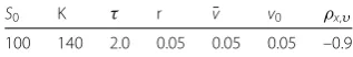
Table 1 Deterministic parameter setting for the put option
S0 K τ r ¯v v0 ρx,υ
100 140 2.0 0.05 0.05 0.05 –0.9
If we focus on pricing a financial instrument, such as a put option, for every sample of the parameters involved in the mathematical model governing the price of the product, we will obtain a value given by the chosen numerical solver. Then, the propagation of the uncertainty from the model parameters to the output is dominated by the computational cost of the numerical solver. Due to this, it is important to choose an efficient numerical method with a low computational cost. In this work, put options have been considered (Table1) but exotic financial products could also be taken such as variance swaps or cliquet options.
3.1 Tests
Among the whole set of possible random parameters,κ,υ¯ andγ have an important role as they are involved in the Feller condition. As a first approach and in order to simplify the results to visualize some conclusions, only parametersκandγ have been considered. Thus, we obtain a two-dimensional problem for UQ. Tests where Feller condition is satis-fied or not have been carried out. The numerical results shown in this section will give us an insight in the impact of the variability ofκandγ on the output of the stated problem. All the computations have been done for timeτ= 2 and the deterministic values for the parameters can be seen in Table1.
The probability distribution of the uncertain parameters has to be fixed as the Stochastic Collocation method is based on a transformation to an artificial space. Then the colloca-tion points are computed in this new stochastic space whose properties are already known and the probability of the solution is built with Lagrange interpolation. In previous works like [7] the exponential convergence of the Stochastic Collocation method is shown for uniformly distributed uncertain parameters so in this work, uniform distribution has been chosen to generate the random parameters.
The results have been computed using nine interpolation points in each direction of the domain, that is eighty-one collocations points (Fig.1(a)). However, having in mind a higher dimensional problem, a Smolyak approximation has been considered in order to reduce the computational time so the number of points is reduced to twenty-nine (Fig.1(b)). Al-though in this case the improvement is not very noticeable, an important time reduction is expected for higher dimensions, because an increase of the number of uncertain param-eters turns into an increase of the number of collocation points where the approximate solution is computed by the COS-method.
3.1.1 Test1:Feller condition satisfied
Figure 1Stochastic Collocation points for full and sparse grids
Figure 2Results for Test 1 (Feller condition satisfied)
the values in the whole domain, the Lagrange interpolation has been used. In Fig.2(c)–(d) the standard deviations for the implied volatility and put prices are depicted.
3.1.2 Test2:Feller condition not satisfied
Figure 3Results for Test 2 (Feller condition not satisfied)
3.1.3 Test3:mixed Feller condition
We are also interested in cases where a mixed Feller condition holds. In the numerical results to follow,κwill vary in [0.4, 11.0] andγ in [0.05, 0.5]. Thus, the Feller condition can be either satisfied or not at sample points considered in these domains. In this case where the Feller condition is satisfied at some points of the domain considered forκand
γ, we see a highly satisfactory performance of the interpolation method in Fig.4(a)–(b) as in previous subsections. It is remarkable that the behaviour is completely different from the ones shown in previous cases. This should be related to the strestch range of values of the parameters. In Fig.4(c)–(d) the standard deviations for the implied volatility and put prices are shown.
After having an insight in the three cases we can describe some conclusions. If the Feller condition is satisfied, the implied volatility and the put price increase with increasingκand decreasingγ. The response surface is close to linear, despite the large parameter domain. When the Feller condition is not satisfied, the response is much more nonlinear. For the mixed Feller condition case, the response is even more nonlinear being partly caused by the largest parameter ranges used. For the cases with the Feller condition satisfied, and not satisfied, the standard deviation converges quickly whereas the convergence is slower for the mixed Feller condition case, because of the nonlinearity of the response. The standard deviation of the nonlinear solution for the case Feller not satisfied is smaller than for the case Feller satisfied, being the input uncertainty in the former case smaller. However, the standard deviation for the mixed case is highest.
3.2 Numerical test with real market data
Figure 4Results for Test 3 (Mixed Feller condition)
Figure 5Spot values of the Eurostoxx50
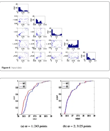
Figure 6Input data
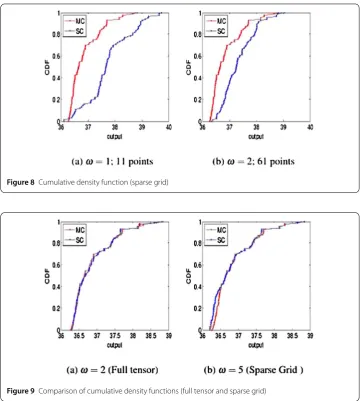
Figure 7Cumulative density function (full tensor)
The computational cost is about 8 minutes as the Smolyak approximation is considered for the post-processing where stochastic collocation method is involved. Throughout this test the put option deterministic parameters are the same as the ones of the previous an-alytical tests collected in Table1.
The cumulative probability distribution function (CDF) of the put option prices is com-puted by a Monte Carlo simulation of the data points and by the Stochastic Collocation method as we can see in Fig.7to10. In Fig.7and8, the approximations for levelω={1, 2} are shown. Both the number of points and the accuracy of the tensor product grid approx-imation increases faster withω. In Fig.9the approximations for the full tensor for level
Figure 8Cumulative density function (sparse grid)
Figure 9Comparison of cumulative density functions (full tensor and sparse grid)
Figure 10 Comparison of cumulative density functions (sparse grid)
The convergence behavior is compared in Tables2and3with the Monte Carlo solution as function of the level ωand the number of points. The mean and standard deviation are integral quantities and therefore the mean and standard deviation errors can converge non-monotonically due to cancellation of errors. TheL1error is added as a stronger
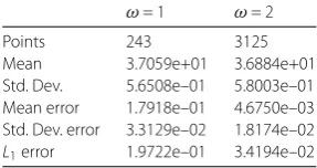
Table 2 Convergence full tensorω= 1, 2. Monte Carlo solutions mean 3.6879e+01 and standard deviation 5.9820e–01
ω= 1 ω= 2
Points 243 3125
Mean 3.7059e+01 3.6884e+01
Std. Dev. 5.6508e–01 5.8003e–01 Mean error 1.7918e–01 4.6750e–03 Std. Dev. error 3.3129e–02 1.8174e–02 L1error 1.9722e–01 3.4194e–02
Table 3 Convergence sparse gridω= 1, 2, 3, 4, 5. Monte Carlo solutions mean 3.6879e+01 and standard deviation 5.9820e–01
ω= 1 ω= 2 ω= 3 ω= 4 ω= 5
Points 11 61 241 801 2433
Mean 3.7765e+01 3.7338e+01 3.6779e+01 3.6926e+01 3.6842e+01
Std. Dev. 8.5236e–01 6.0479e–01 6.8795e–01 5.94229e–01 6.1646e–01
Mean error 8.8542e–01 4.5846e–01 9.9622e–02 4.6040e–02 3.7463e–02
Std. Dev. error 2.5416e–01 6.5885e–03 8.97506e–02 3.9754e–03 1.8257e–02
L1error 9.0194e–01 4.6129e–01 1.4612e–01 5.5369e–02 4.9122e–02
The conclusion of this section is that the accuracy of the sparse grids interpolation tech-nique is comparable to that of the full tensor grids as function of the number of points. The additional advantage of sparse grids is that the number of points grows more slowly with the level than the full tensor grids, such that more convergence information and smaller point sets are available. Levelsω= 1 andω= 2 of the full tensor should therefore be com-pared to the sparse grids on levelsω= 3 andω= 5 with approximately the same number of points, respectively. In this case, the number of points for most of the levels is larger than the 84 data points in the Monte Carlo simulation. However, the number of computa-tions in the Stochastic Collocation method is independent of the number of data points. Stochastic Collocation could therefore be faster than Monte Carlo simulation at an ac-ceptable accuracy, in cases in which a larger set of market data points is available.
The good performance of the method is seen as both cumulative density functions are close one to each other.
4 Conclusions
The impact of the uncertainty provided by the randomness of the parameters in the Hes-ton model is studied by means of Uncertainty Quantification. In particular, the Stochastic Collocation Method is used to study the propagation of the uncertainty from the input of the model to the solution.
It is challenging to apply techniques already used in fluid dynamics to computational finance and on the other hand, the good performance of this kind of methods is stated through the tests considered in this paper. Firstly, the analytical tests show an insight of the impact of the variability ofκandγ on the output of the problem. If the Feller condition is satisfied, the response surface is close to linear but if Feller condition is not satisfied, the response is much more nonlinear. For mixed Feller condition, due to the largest parameter range, the response is even more nonlinear and the standard deviation is largest than for the tests where Feller condition is satisfied.
con-sequence, despite suffering from the curse of dimensionality as the number of collocation points also increases, Smolyak sparse grid Stochastic Collocation Method is used to re-duce the computational cost of the method.
Having in mind the importance of the calibration and hedging procedures, the study of the impact of uncertain parameters on the Greeks and the distribution of the model parameters would make pricing more reliable. Furthermore, it would be interesting to extend these studies to exotic products such as variance swaps and cliquet options.
Acknowledgements
Not applicable.
Funding
This paper has been ERCIM “Alain Bensoussan Fellowship Programme” and partially funded by MCINN (Project MTM2010–21135–C02-01).
Abbreviations
Implied vol., Implied volatility; Std. Dev., Standard Deviation; UQ, Uncertainty Quantification.
Availability of data and materials
Data sharing not applicable to this article as no datasets were generated or analysed during the current study.
Competing interests
The author declare that they have no competing interests.
Authors’ contributions
All authors were involved in planning the work, drafting and writing the manuscript. Discussion and comments on the results and the manuscript as well as a critical revision have been made by all the authors at all stages. All authors read and approved the final manuscript.
Author details
1Department of Mathematics and CITIC, University of A Coruña, A Coruña, Spain.2CWI—Center for Mathematics and
Computer Science, Amsterdam, The Netherlands.3DIAM, Delft University of Technology, Delft, The Netherlands.
Publisher’s Note
Springer Nature remains neutral with regard to jurisdictional claims in published maps and institutional affiliations.
Received: 23 February 2018 Accepted: 26 June 2018 References
1. Achdou I, Pironneau O. Computational methods for option pricing. Philadelphia: SIAM; 2005.
2. Fang F, Oosterlee CW. A novel pricing method for European options based on Fourier-cosine series expansions. SIAM J Sci Comput. 2008;31:826–48.
3. Fang F, Oosterlee CW. Pricing early-exercise and discrete-barrier options by Fourier-cosine series expansions. Numer Math. 2009;114:27–62.
4. Glasserman P. Monte Carlo methods in financial engineering. Berlin: Springer; 2003.
5. Heston S. A closed-form solution for options with stochastic volatility with applications to bond and currency options. Rev Financ Stud. 1993;6:327–43.
6. Loeven GJA, Witteveen Jeroen AS, Bijl H. Probabilistic collocation: an efficient nonintrusive approach for arbitrarily distributed parametric uncertainties. In: 45th AIAA Aerospace Sciences Meeting and Exhibit. Reno, Nevada. 7. Loeven GJA, Witteveen Jeroen AS, Bijl H. (Student paper) Efficient Uncertainty Quantification in Computational
Fluid-Structure Interaction. In: Proceedings of the 8th AIAA Non-Deterministic Approaches Conference. Newport. AIAA paper 2006-1634.
8. Marcozzi MD. On the valuation of Asian options by variational methods. SIAM J Sci Comput. 2003;24:1124–40. 9. Nobile F, Tempone R, Webster CG. A sparse grid stochastic collocation method for partial differential equations with
random input data. SIAM J Sci Numer Anal. 2008;46:2309–45.
10. Smolyak SA. Quadrature and interpolation formulas for tensor products of certain classes of functions. Dokl Akad Nauk SSSR. 1963;4:240–3.
11. Trefethen LN. Is Gauss quadrature better than Clenshaw–Curtis? SIAM Rev. 2008;50:67–87.