Parametric modeling and model order reduction for (electro-)thermal analysis of nanoelectronic structures

(1)

R E S E A R C H

Open Access

Parametric modeling and model order

reduction for (electro-)thermal analysis of

nanoelectronic structures

Lihong Feng

1

_{, Yao Yue}

1*

_{, Nicodemus Banagaaya}

1

_{, Peter Meuris}

2

_{, Wim Schoenmaker}

2

_and

Peter Benner

1

*_{Correspondence:}

[email protected] 1_{Max Planck Institute for Dynamics}

of Complex Technical Systems, Sandtorstr. 1, Magdeburg, 39106, Germany

Full list of author information is available at the end of the article

Abstract

In this work, we discuss the parametric modeling for the (electro)-thermal analysis of components of nanoelectronic structures and automatic model order reduction of the consequent parametric models. Given the system matrices at diﬀerent values of the parameters, we introduce a simple method of extracting system matrices which are independent of the parameters, so that parametric models of a class of linear parametric problems can be constructed. Then the reduced-order models of the large-scale parametric models are automatically obtained usinga posteriorioutput error bounds for the reduced-order models. Simulations of both thermal and electro-thermal systems conﬁrm the validity of the proposed methods.

1 Introduction

Parameter variations have become essential in the design of micro- and nano-electronic (-mechanical) systems as well as of coupled electro-thermal problems, since in many anal-yses such as optimization and uncertainty quantification, modeling and simulation at many values of the parameters are unavoidable. For many design and analysis tools, mod-eling and simulation need to be done at each instance of the parameter from scratch: given a fixed value of the parameter, sayp∗, a certain numerical discretization method, e.g., a fi-nite element method, is used to build a spatially discretized model only valid forp∗, and numerical integration is then performed to get the output response corresponding top∗. If additional analysis beyond the capability of the aforementioned software is required, the software often can provide only the (conductivity, capacitance) matrices corresponding to certain samples of the parameter, rather than explicit matrix functions that are more convenient for mathematical analysis.

It is desired to derive a single parametric discretized system that is valid for all pos-sible values of the parameters, so that discretization does not have to be implemented anew for each value of interest, which can save much simulation time. In this paper, we propose a simple method of extracting matrix functions that is capable of calculating the matrices corresponding to any parameter value efficiently. Thanks to these matrix func-tions, the dynamics of the parametric system can be described by a single system of para-metric ordinary differential equations (ODEs) or differential-algebraic equations (DAEs).

(2)

The approach is in particular suitable for the (electro)-thermal analysis of nanoelectronic structures, as the parameters there often appear in a linear aﬃne form required by this extraction for a parametric model.

Simulating the consequent parametric system is, however, still very time consuming, because of the high dimension of the system. We propose to use parametric model order reduction (PMOR) to compute a reduced-order model (ROM) that is not only of a much lower dimension, but also accurate for all values of the parameters within a specified range. Therefore, using the parametric ROM to replace the full-order model (FOM) in simulation and other analyses like optimization and uncertainty quantification leads to significant speedup and high accuracy. Many PMOR methods have been proposed so far. A survey of PMOR methods can be found in []. In this paper, we use a multi-moment-matching PMOR method [] to construct the reduced-order model. These methods are popular in practical applications since they are easy to implement, need less computations than most of the other methods, and are therefore suitable to reduce high-dimensional ODE/DAE systems that commonly arise in design and analysis of VLSI (very-large-scale integration) circuits. Furthermore, we propose to use ana posteriorioutput error bound [] to con-struct the ROM automatically, i.e., the algorithm can build a reduced-order model satisfy-ing a prescribed error tolerance without further specification of algorithmic parameters, e.g., interpolation points and the order of the ROM, which can be automatically deter-mined by the algorithm in an adaptive manner.

The paper is organized as follows. In Section , we propose a simple method of extract-ing the state-space representation of a class of parametric problems. Section  reviews the basic idea of PMOR methods and Section  describes an algorithm that implements the multi-moment-matching PMOR method adaptively based on ana posteriorioutput er-ror bound for the ROM. Section  describes the (electro-)thermal simulation for two test models: a package model and a Power-MOS device model. The parametric modeling and PMOR of these models, especially the extraction of the tensors and PMOR for the one-way nonlinearly coupled dynamical system, are discussed in Section . The numerical results are presented in Section , and the paper is concluded in Section . In all test cases, the matrices are eﬃciently extracted and the parametric ROMs automatically obtained meet the requirements on accuracy and compactness.

2 Parametric modeling

In this section, we introduce a method for extracting system matrices of a class of para-metric problems, so that the parapara-metric representation of the models in state-space form can be derived. Assume that the parametric problem can be generally described by the following partial diﬀerential equation,

∂a(t,z;p) ∂t +L

a(t,z;p)=f(t,z;p), t∈[,T],z∈,p∈P, ()

whereL[·] is a linear spatial diﬀerential operator,f(t,z;p) is the excitation,p= (p, . . . ,pm)T

is a vector of parameters, ⊆Rd (d= , , ) is the spatial domain andP ⊆Rm _{is the}

parameter domain.

(3)

exerted on the contacts (inputs). In such cases, state-space representation is often used for the spatially discretized system. Using ﬁnite-element simulation software, we can usu-ally conduct spacial discretization only at a ﬁxed valuep∗ofpand obtain the discretized system

Ep∗dx(t,p

∗₎

dt =A

p∗xt,p∗+Bp∗u(t), yt,p∗=Cp∗xt,p∗+Dp∗u(t),

()

where only E(p∗),A(p∗)∈Rn×n,B(p∗)∈Rn×lI_, _C₍_p∗₎∈RlO×n_{, and}_D₍_p∗₎∈RlO×lI _{at the}

ﬁxed valuep∗ofpare available. Here,x∈Rn_{is the state vector, and}_y_∈_RlO_{is the output}

response. For design purposes, the simulation results at many ﬁxed values ofpshould be derived and analyzed. If we simply use the software, the discretization must be repeated at many values ofp. To avoid repeated discretization in space, and hence to save design time, it is desired that a parametric representation of the model is available.

We will show that ifE(p),A(p),B(p),C(p),D(p) are in the form of

M(p) =pM+· · ·+pmMm, ()

we can easily computeM, . . . ,Mmbased on the data ofM(p) atmﬁxed values ofp(here

and below, M(p) stands for any of the matrices E(p),A(p),B(p),C(p),D(p)). Hence, the parametric representation of () is available, i.e.,

E(p)dx(t,p)

dt =A(p)x(t,p) +B(p)u(t),

y(t,p) =C(p)x(t,p) +D(p)u(t).

()

The discretized parametric model in () not only prevents repeated discretization at all values ofp, but also retains the same system ordern as the nonparametric system () regardless of the number of the parameters. Note that the linear-aﬃne form () does not require linear dependence on geometrical and/or physical parameters sincepimay present

abstract parameters. It covers a rather broad range of applications since any system of the form

M(q) =φ(q)M+· · ·+φm(q)Mm, ()

whereφirepresents an arbitrary scalar function ofq, can easily be rewritten into form ()

with the change of parameterpi=φi(q). The vectorspandqcan be of diﬀerent lengths,

e.g., for the package model that will be described in Section , we setp= ,p=h,p=_h, wherehis the top layer thickness of the package. Note that any parametric matrixM(q) can be written into the form () theoretically since if we denote the (i,j)-th entry ofM(q) bymi,j(q),M(q) can be at least expanded as

M(q) =

n

i=

n

j= mi,j(q)

eieTj

(4)

whereeiis thei-th column of then×nidentity matrix. In practice, however,min ()

should be small enough, e.g., below ten, if PMOR is expected to be efficient on the ex-tracted system. A concise form can often be obtained by physical reasoning provided by engineers. For our test examples in Section ,M(h) =M+hM+_hMwhen the thick-ness parameter hchanges, andM(σ) =M+σM when the conductivity parameterσ changes. However, there are still cases where the space-discretization does not yield a concise affine-linear structure. For such cases, empirical interpolation method [, ] is commonly applied to obtain an approximation with an affine structure.

Suppose that m groups of matrices E(pai_),_A₍_pai_),_B₍_pai_),_C₍_pai_),_D₍_pai_{) have been}

ob-tained, e.g., by simulation software atmdiﬀerent samplespai_,_i_{= , . . . ,}_m_{. Using the}

for-mulation in (), one can get a group of equations as below,

pa_ M+· · ·+pamMm=M

pa_,

.. .

pam

 M+· · ·+pammMm=M

pam_.

()

The equations above can be re-written as

(Pm⊗In)

⎛ ⎜ ⎜ ⎝ M .. . Mm ⎞ ⎟ ⎟ ⎠= ⎛ ⎜ ⎜ ⎝

M(pa) .. . M(pam₎

⎞ ⎟ ⎟

⎠, ()

whereIn∈Rn×nis the identity matrix, and

Pm=

⎛ ⎜ ⎜ ⎝

pa . . . p

a m

..

. ... pam

 . . . pamm

⎞ ⎟ ⎟

⎠∈Rm×m.

Ifp,p, . . . ,pmare independent parameters, it is possible to select the samplespai such

that the correspondingm×mmatrixPm in () is nonsingular, since otherwise, one or

more parameters can be removed. Under this assumption,

⎛ ⎜ ⎜ ⎝ M .. . Mm ⎞ ⎟ ⎟

⎠=P_m–⊗In

⎛ ⎜ ⎜ ⎝

M(pa₎

.. . M(pam₎

⎞ ⎟ ⎟ ⎠,

where we use the following property of the Kronecker product: (U⊗Q)–₌_U–_⊗_Q– for any nonsingular matricesU∈RnU×nU _and_Q∈RnQ×nQ _{[]. Finally, the matrices}_M

i

(i= , . . . ,m) can be easily computed by

M=p˜M

pa+· · ·+p˜mM

pam_,

.. .

Mm=p˜mM

pa+· · ·+p˜mmM

pam_,

(5)

wherep˜ijis the (i,j)-th entry of the matrixP–m:

P–_m = ⎛ ⎜ ⎜ ⎝

˜

p . . . p˜m

..

. ...

˜

pm . . . p˜mm

⎞ ⎟ ⎟

⎠. ()

An important property of the computation above is that it is independent of the large di-mensionn(typically several thousands or even higher) in linear system solves. To compute allMi(Mi=Ei,Ai,Bi,Ci,Di,i= , . . . ,m) in () for any large-scale matrices in (), we need

only to invert a small-scalem×mmatrixPm once (mis typically below ten and equals

 or  in our numerical examples) and conduct scalar-matrix multiplication and matrix addition with the dimensionn, all of which are computationally much more eﬃcient than solving () with its ordermn. Note that the full inverse for such a small matrix can readily be computed, and multiplication with it is somewhat faster than working with the trian-gular factor and backward/forward solves due to the memory access pattern.

Simulating the system in () may still take a lot of time when the dimensionnis large, especially when it has to be simulated at many samples ofp(like in optimization). In the next section, we propose to use PMOR to construct a parametric reduced-order model, which will replace the original large-scale system in () in simulations for speedup. Since the size of the reduced-order model is usually much smaller thann, simulation can be conducted within a much shorter and more reasonable time period.

3 PMOR based on multi-moment-matching

Various PMOR methods have been proposed in the literature, among which the meth-ods based on multi-moment-matching are probably the easiest to implement and the most computationally eﬃcient for many applications, especially for linear systems []. The multi-moment-matching PMOR method computes a basis matrixV based on the series expansion of the state vectorxin the frequency domain. Under the zero initial condition, the frequency domain description for system () is

sE(p) –A(p)x(s,p) =B(p)u(s),

y(s,p) =C(p)x(s,p) +D(p)u(s), ()

where we assume that the matrix pencil (A(p),E(p)) is regular for anypvalue, i.e., there ex-istsλp,such thatλp,E(p) –A(p) is nonsingular. Given expansion pointsp= [p, . . . ,pm],

ands,x(s,p) in () can be expanded as

x(s,p) =I– (σG+· · ·+σmGm+σm+Gm++· · ·+σmGm)

– BMu(s)

=

∞

i=

(σG+· · ·+σmGm)iBMu(s), ()

where σi =spi –spi, σm+i =pi–pi, Gi = –[sE(p) –A(p)]–Ei, Gm+i = [sE(p) – A(p)]–Ai,i= , , . . . ,m, andBM= [sE(p) –A(p)]–B(p), under the condition that all matrices in [·]–are nonsingular and

(6)

Because of condition (), the resulting ROM is normally accurate only around the expan-sion pointp_{. To obtain a parametric ROM valid on a wider range, multiple expansion} points are often employed as we will show below.

Deﬁning

Rj= [G, . . . ,Gp]Rj–, j= , . . . ,q,

and

R=

sE

p–Ap–[B, . . . ,Bm],

we can compute the matrix Vs,p_,_q, whose columns form an orthonormal basis of the

subspace spanned by the ﬁrstqofRi’s:

range{Vs,p_,_q}=span{R_,R_, . . . ,R_q}_s_,_p. ()

UsingV :=Vs,p_,_q, which is assumed to be ann×n_rmatrix, we obtain the parametric

reduced-order model via Galerkin projection,

VTE(p)Vdxr(t,p)

dt =

VTA(p)Vxr(t,p) +

VTB(p)u(t),

yr(t,p) =

C(p)Vxr(t,p) +D(p)u(t),

()

where the state vectorxr(t,p) is of ordernr. WhenA(p),B(p),C(p),E(p) all take the aﬃne

form (), the reduced parametric matrices can be computed by the formula

VTE(p)V=pVTEV+· · ·+pmVTEmV,

VTA(p)V=pVTAV+· · ·+pmVTAmV,

VT_B₍_p_{) =}_p

VTB+· · ·+pmVTBm,

C(p)V=pCV+· · ·+pmCmV,

where all constant matrices on the right-hand side can be pre-computed.

Note that the number of columns inRjincreases exponentially withj. When the number

of the parameters inpis larger than , or when there are many inputs, multiple expansion points should be used to keep the size of the reduced-order model reasonable. The idea is straightforward. Given a set of expansion pointssi,pi,i= , . . . ,k(the superscriptiforp

is not a power: it only indicates thei-th expansion point), a matrixV_s_i_,_pican be computed

for each pair (si,pi) as

range{Vsi,pi,qr}=span{R,R, . . . ,Rqr}si,pi. ()

The ﬁnal projection matrix V is obtained from the orthogonalization of all matrices V_s_i_,_pi_,_q_r,

V=orth{Vs,p_,_q

(7)

For similar accuracy, the numberqrin () can usually be taken much smaller thanqin ()

and normally, only a few well-chosen expansion points suﬃce. For example,  or  com-monly suﬃces forqr, whileqmust be taken a much larger value depending on the problem.

The reason is that, using multiple expansion points, the diﬃculty of the parametric depen-dence can be tackled by adding new interpolation points, each of which adds only a few columns due to the smallqr, which is much more economical than using a single expansion

point, where this diﬃculty must be treated with the increase ofq, each step of which be-comes increasingly more expensive. Consequently, the reduced-order model is normally smaller and more accurate on a broader parameter range when multiple expansion points are used.

The choice of the number and locations of the expansion points (si,pi) has an important

inﬂuence on the eﬃciency of multi-moment-matching PMOR methods. Actually, good accuracy and compactness of the reduced-order model can only be achieved when the expansion points are selected judiciously.

In the next section, we introduce a technique for adaptively selecting the expansion points according to ana posteriorierror bound(s,p) for the ROM. By using the error bound to access the reliability of the reduced-order model, we develop an automatic pro-cedure for constructing the ROM.

4 Adaptively selecting the expansion points

For the general system () withlIinputs andlOoutputs, the error bound(s,p) is deﬁned as

(s,p) = max ≤i≤lI, ≤j≤lO

ij(s,p),

whereij(s,p) is the error bound for the (i,j)-th entry of the transfer function matrix of

the ROM, i.e.,

Hij(s,p) –Hˆij(s,p)≤ij(s,p),

whereH(s,p) andHˆ(s,p) represent the transfer functions of the full-order model and the reduced-order model, respectively. In this paper, we deﬁne theij(s,p) as in [], which is

inspired by thea posteriorierror bounds proposed for the reduced basis method []:

ij(s,p) =

rdu_i (s,p)rjpr(s,p) β(s,p) +xˆ

du∗_rpr j (s,p),

where

rpr_j (s,p) =B(:,j) – [sE–A]xˆpr_j ,

ˆ

xpr_j =VsVTEV–VTAV–VTB(:,j),

rdu_i (s,p) = –C(i, :)T–¯sET–ATxˆdu_i ,

¯

sis the conjugate ofs, and the statexdu_i of the dual system is approximated by

ˆ

(8)

Here, for ease of notation,pis dropped from the matricesE(p),A(p),B(p) andC(p), and thej-th column ofB(p) and thei-th row ofC(p) are denoted byB(:,j) andC(i, :), respec-tively. The variableβ(s,p) is the smallest singular value of the matrixsE(p) –A(p). The matrixVdu can be computed, for example, using () and (), but replacingR, . . . ,Rqr

withRdu_ ,Rdu_ , . . . ,Rdu

qr, where the matricessiE(p

i_{) –}_A₍_pi_{) in}_R

, . . . ,Rqr are substituted by ¯

siET(pi) –AT(pi), andEjbyETj ,AjbyATj ,BjbyC(j, :)T,j= , . . . ,m. The derivation of(s,p)

is detailed in [].

Algorithm Adaptively selecting expansion pointsˆs,pˆ, and computingVautomatically

: V= [];Vdu_{= [];}

: Choose someεtol<  and a small positive integerqr; setε= ;

: Choosetrain: a large set of samples ofsandp, taken over the domain of interest;

: Choose the initial expansion point: (ˆs,pˆ);

: whileε>εtoldo

: range(Vˆs,pˆ,qr) =span{R,R, . . . ,Rqr}ˆs,pˆ;

: range(V_ˆ_sdu_,_p_ˆ_,_q

r) =span{R

du

 ,Rdu , . . . ,Rqdur}ˆs,pˆ;

: V=orth{V,Vsˆ,pˆ,qr};

: Vdu=orth{Vdu,V_s_ˆdu_,_p_ˆ_,_q_r}; : (ˆs,pˆ) =arg maxs,p∈train(s,p);

: ε=(sˆ,pˆ) ;

: end while.

Thanks to the error bound(s,p) for the ROM, the expansion points (si,pi) can be

se-lected adaptively, and the projection matrixVcan be computed automatically as is shown in Algorithm . It is worth pointing out that although the error bound is parameter-dependent, many p-independent terms constituting the error bound need to be pre-computed only once, which can be repeatedly used in the algorithm for all samples of pintrain, e.g., the termsVTMV, . . . ,VTMmV, etc.

5 Test models

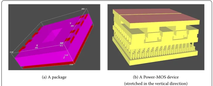
To test the techniques proposed, we will use two applications arising from thermal and electro-thermal simulations: a package shown in Figure (a), whose purpose is to allow easy handling and assembly onto printed circuit boards and to protect the devices from damage [], and a Power-MOS device shown in Figure (b), which is commonly used in energy harvesting, where energy from external sources like light and environmental heat is collected in order to power small devices such as implanted biosensors [, ]. With the scaling down of integrated circuits, thermal issues have attracted increasingly more attentions and become a major consideration in the design of integrated circuits.

The dynamics of both applications can be described by the same governing equations. The electrical sub-system can be described by

∇ ·J+∂ρ ∂t = ,

J=σ·E, E= –∇U,

(9)

(a) A package (b) A Power-MOS device (stretched in the vertical direction)

Figure 1 Physical models considered in the numerical tests.

whereJis the current density,Eis the electrical field,Uis the electrical potential,σis the electrical conductivity,is the permittivity, andρis the charge density. In this paper, we ignore both the local charging, i.e.,=  andρ= , and the dependence of the electrical conductivityσon temperature, i.e., the electrical sub-system is independent of the thermal sub-system, and obtain the following simplified governing differential equation, which is time-independent:

∇ ·(σ· ∇U) = .

The thermal sub-system is governed by similar equations:

∇ ·φq+

∂w(T) ∂t =Q,

φq= –κ∇T,

w(T) =CT(T–Tref),

where φq is the heat ﬂux,wis the local energy storage,CT is the thermal capacitance,

andQrepresents heat sources or sinks. For the thermal sub-system, we also ignore the dependence of the thermal capacitance on the temperature. ForQ, we use two options in this paper.

•The thermal-only option takesQas an independent input. Under this option, the elec-trical sub-system and the thermal sub-system are completely decoupled. The thermal-only option is especially interesting to the package model, since it can be used to study the thermal dynamics stimulated by heat-injecting or extracting properties on the bound-ary of the simulation domain, Joule self-heating, etc. Finite element discretization of the thermal-only option leads to a linear dynamical system exactly the form ().

•The electro-thermal option takesQas a coupling term from the electrical sub-system: the Joule self-heating that is of great importance in power-aware design of integrated cir-cuits:

(10)

In this case, the whole system is one-way coupled: the thermal sub-system depends on the electrical sub-system, while the electrical sub-system is independent of the thermal system. The state space representation of the electro-thermal option is:

⎧ ⎪ ⎪ ⎪ ⎪ ⎪ ⎪ ⎪ ⎪ ⎨ ⎪ ⎪ ⎪ ⎪ ⎪ ⎪ ⎪ ⎪ ⎩

AE(p)xE(t,p) = –BE(p)u(t), (a)

ET(p)x˙T(t,p) =AT(p)xT(t,p) +BT(p)u(t) +F(p)×xE(p)×xE(p), (b)

xT(,p) =xT, xE(,p) =xE, (c)

y(t,p) =CE(p)xE(t,p) +CT(p)xT(t,p) +D(p)u(t), (d)

where the input vector u∈RlI _{represents the input voltages and temperatures at the}

contacts, the output vector y∈RlO _{represents the output voltages, currents,}

tempera-ture, and thermal ﬂuxes at the contacts,AE(p)∈RnE×nE,BE(p)∈RnE×lI,ET(p)∈RnT×nT, AT(p)∈RnT×nT, BT(p)∈RnT×lI, CE(p)∈ RlO×nE, CT(p)∈RlO×nT, DT(p)∈RlO×lI, and the tensorF(p)∈RnT×nE×nE_{, which can be considered as}_n

T slices ofnE by nE matri-cesFi(p)∈RnE×nE, i= , . . . ,nT, represents the nonlinear coupling of the electrical part with the thermal part. Denoting thei-mode tensor-matrix product by×i[], the

prod-uctF(p)×xE(p)×xE(p) is a vector of lengthnT, whosei-th component is the standard vector-matrix-vector productxE(p)TFi(p)xE(p). In this formulation, the algebraic equa-tion (a) describes the electrical part, the ordinary differential equaequa-tion (b) describes the thermal part, in which the tensorF(p) describes Joule self-heating, (c) specifies the initial conditions, and (d) computes the output obtained from the electrical and thermal state vectors. Theoretically, Joule self-heating should be modeled by two tensor products: F(p)×xE(p)×xE(p) andG(p)×xE(p)×u(t). However, the influence of the second part is rather limited, and is therefore ignored in this paper. Instead of a single coupled system, we write out the electrical and thermal sub-systems explicitly to show the one-way coupling. Furthermore, our numerical results proved that PMOR is computationally much more efficient if we apply it to the algebraic equations and the ordinary differential equations separately rather than apply it to a single set of differential algebraic equations.

6 Parametric modeling and PMOR for the test models

For the package model shown in Figure (a), the parameterp is chosen to be the top layer thickness of the package, namelyh. The finite-integration technique (FIT) for the modeling of the package leads to thermal fluxes that are proportional to the dual areas of the mesh cells and inversely proportional to the lengths of the edges in the mesh cells. Therefore, when considering meshes that are topologically equivalent for different pack-age thicknesses, the parametric dependence of the matrices will take the form

M(h) =M+hM+ 

hM (M=AE,BE,ET,AT,BT,F,CE,CT,D).

(11)

Note that the method developed in Section  also applies to the tensorF due to the following reasoning. Every slice ofF, sayFi(p)∈RnE×nE, can be extracted using the

proce-dure from () to (), and under the same set of samplespa_,_pa_{, . . . ,}_pam_{in (), the obtained}

coeﬃcientsp˜,p˜, . . . ,p˜mmin () are the same. Therefore, the computation for all slices

can be conducted together in the tensor form, i.e., assuming thatM,M, . . . ,Mmin () are

tensors, they can be extracted by (), using the coeﬃcient computed by ().

Therefore, to extract all matrices and tensors for the package model, we need ﬁrst only to invert a single × matrix, and then, for each matrix or tensor function, we need to calculate () once.

For the Power-MOS circuit model shown in Figure (b), the conductivity of the third metal layer, which we denote byσ, is chosen to be the parameter. The ﬁnite-integration technique (FIT) assembles ﬂuxes that are proportional to the conductivity of each mesh cell material, and therefore, the parametric dependence of the matrices will take the form

M(σ) =M+σM (M=AE,BE,ET,AT,BT,F,CE,CT,D).

It is clearly in the form () by assigningp=  andp=σ, and the proposed procedure for extracting the matrices/tensors can readily be used.

The remaining problem is how to reduce system (b), which has a quadratic one-way coupling term. To simplify the presentation, we use the Power-MOS circuit with the pa-rameter dependenceM(σ) =M+σM as an example. Following the idea presented in [], we ﬁrst ignore the nonlinear partF(p)×xE(p)×xE(p) in system (b) and use the adaptive PMOR algorithm proposed to reduce the resulting system in the form () [, ]. To approximate the one-way coupling term, we need to reduce the electrical sub-system before the thermal sub-system.

•The electrical sub-system (a) is already in the form () if we assignE(p) = ,A(p) = –AE(p),B(p) = –BE(p),s=t, by noting that for the validity of the proposed PMOR method, system () is actually not necessarily a frequency-domain system. Denote the basis built for the electrical sub-system (a) byVE. For MOR for algebraic equations, it is worth mentioning the exact reduction method proposed in [] for non-parametric systems, which does not require an error bound. However, the method we propose in this paper can not only reduce parametric systems, but also normally build a reduced-order model of a much lower dimension.

•If we ignore the nonlinear coupling term in the thermal sub-system (b), it is already in the form (). To use the methods developed, we ﬁrst conduct the Laplace transform to obtain its frequency domain representation

AT+σAT–sET– (σs)ET

X=BTBTATxTATxT

⎡ ⎢ ⎢ ⎢ ⎣

–U –σU

–

s

–σ

s

⎤ ⎥ ⎥ ⎥

⎦. ()

Then, we apply Algorithm  to system () to obtain the basis for the thermal sub-system, which we denote byVT.

(12)

ROM is

ET(p)x˙T(t,p) =AT(p)xT(t,p) +BT(p)u+F(p)×xE(p)×xE(p), ()

whereET(p) =VTTET(p)VT,AT(p) =VTTAT(p)VT,BT(p) =VTTBT(p),F(p) =F(p)×VT× VE×VE. To obtain the reduced tensorF(p), we ﬁrst approximatexE(p) in the range of VE, and then project the approximation onto the test subspaceVT, i.e., the tensor product F(p)×xE(p)×xE(p) equalsVTT[F(p)×(VExE(p))×(VExE(p))]. The advantage of the tensor formulation for the ROM is that using the reduced tensor, evaluating the ROM does not require computations with quantities of the order of the FOM. In our actual computations, the parametric matrices in the ROM are computed by

Y(p) =Yc+pYv, Y∈ {AT,BT,CT,ET,F}, ()

whereYcandYvare pre-computed during the construction of the ROM. This precompu-tation is also applied to the electrical sub-system (a) and the output compuprecompu-tation (d).

7 Numerical results

In this section, we ﬁrst show the numerical results of the thermal analysis of the package model. Then, we present the numerical results of the electro-thermal analysis of both the package model and the Power-MOS device model.

7.1 Numerical results for the thermal analysis

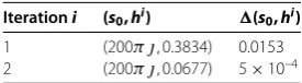
The package model is a multi-input multi-output system, with  inputs and  out-puts. Algorithm  is employed to compute the parametric reduced-order model automat-ically. We used  samples of the package thicknessh∈( μm,  μm], and one sample of s= πfj,f ∈[ Hz, _Hz]:_s

= π j,j =

√

–, to constitute the training settrain in Algorithm . The algorithm essentially selects the expansion points forp, since we ﬁxs to the single expansion points. Only two iterations and two expansion points selected are required for convergence. The reduced-order model is of sizer= . For each selected expansion point, we constructVsi,piwith only two termsRandR(qr=  in Steps -,

Al-gorithm ) in order to avoid the exponential increase inRj,j> . Table  lists the iterations

and the error bounds at each iteration step.

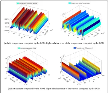
Figure (a) and (b) plot the temperature and the current at two diﬀerent parts of the package, respectively. The temperature is of big magnitude, while the current is of very small magnitude, showing that there is no current at that part of the circuit. The reduced-order model catches the accuracy of both at  samples ofp, and  time steps for each sample.

7.2 Numerical results for the electro-thermal analysis

First, we apply the matrix extraction algorithm and adaptive PMOR method developed to the electro-thermal simulation of the package model with  inputs and  outputs.

Table 1 V_s

i,pi= span{R0,R1}si,pi,i= 1, 2,εtol= 10

–3_,_n_{= 8, 549,}_r_{= 58}

Iterationi (s0, hi) (s0, hi)

(13)

(a) Left: temperature computed by the ROM. Right: relative error of the temperature computed by the ROM

(b) Left: current computed by the ROM. Right: absolute error of the current computed by the ROM

Figure 2 Comparison between FOM-based and ROM-based simulation results of the package model, where both the order-8549 FOM and the order-58 ROM have 34 inputs and 68 outputs.

The system is parameterized by the thickness of the top layer and excited by the inputs:

ui=

⎧ ⎪ ⎪ ⎪ ⎪ ⎪ ⎪ ⎨ ⎪ ⎪ ⎪ ⎪ ⎪ ⎪ ⎩

, i= ,

, ≤i≤,

×_t_{+ ,} _i_{= ,}_t_∈_{[, }–_],  i= ,t> –_,  ≤i≤.

The initial condition for all electrical state variables is  V, and the initial condition for all thermal state variables is ◦C. For the electrical sub-system, the training set is

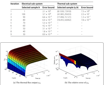
{, , , , , , , , , , , , , }(in μm), while for the thermal sub-system, the training set{(s,h)}contains  samples, in which the frequency (s) and the thick-ness of the top metal layer (h) are uniformly chosen within the ranges [rad_/_s_{, }rad_/_s_{] and} ( μm,  μm], respectively. Using the PMOR method proposed, the electrical sub-system is reduced from order , to order , the thermal system is reduced from order , to order , and the speedup factor for the electro-thermal simulation is .. The con-vergence behavior of the adaptive PMOR method is shown in Table  and the thermal ﬂux outputyand its relative error are shown in Figure .

(14)

Table 2 Convergence behavior of electro-thermal simulation of the package model (_tol= 10–4)

Iteration Electrical sub-system Thermal sub-system

Selected sampleh Error bound Selected sample(s, h) Error bound

1 1 2.1×103 _{(8.1339, 7.5910)} _7.3_×₁₀6

2 100 3.7×100 _{(41.065, 29.653)} _2.3_×₁₀1

3 90 6.6×10–2 _{(17.494, 15.121)} _1.3_×₁₀–1

4 80 6.4×10–3 _{(16.455, 4.6942)} _7.8_×₁₀–5

5 70 5.3×10–3 _– _–

6 60 4.2×10–3 _– _–

7 50 3.1×10–3 _– _–

8 40 1.8×10–3 _– _–

9 30 8.9×10–4 _– _–

(a) The thermal ﬂux outputy (b) The relative error ofy

Figure 3 The thermal ﬂux outputy36and its relative error for the package model.

layer and excited by the inputs:

ui=

⎧ ⎪ ⎪ ⎪ ⎨ ⎪ ⎪ ⎪ ⎩

, i= , ,

_t_, _i_{= ,}_t_∈_{[, }–_], , i= ,t> –_, ., i= , , .

The initial condition for all electrical state variables is  V, and the initial condition for all thermal state variables is . °C. For the electrical sub-system, the training set is

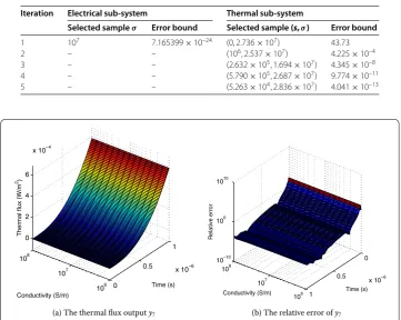
{ S_/_m_{, }_×_ S_/_m_{, }_×_ S_/_m_}_{, while for the thermal sub-system, the training set}_{₍_s_,_σ₎_} contains  samples, in which the frequency (s) and the conductivity of the top metal layer (σ) are uniformly chosen within the ranges [rad_/_s_{, } rad_/_s_{] and [} S_/_m_{, }_×_ S_/_m_], respectively. Using the PMOR methods proposed, the electrical sub-system is reduced from order , to order , the thermal sub-system is reduced from order , to order , and the speedup factor for the electro-thermal simulation is .. The convergence behavior of the adaptive PMOR method is shown in Table  and the thermal ﬂux output yalong with its relative error is shown Figure .

(15)

Table 3 Convergence behavior of electro-thermal simulation of the Power-MOS model (_tol= 10–12)

Iteration Electrical sub-system Thermal sub-system

Selected sampleσ Error bound Selected sample(s,σ) Error bound

1 107 _7.165399_×₁₀–24 _{(0, 2.736}_×₁₀7₎ _43.73

2 – – (106_{, 2.537}_×₁₀7₎ _4.225_×₁₀–4

3 – – (2.632×105_{, 1.694}_×₁₀7₎ _4.345_×₁₀–8

4 – – (5.790×105_{, 2.687}_×₁₀7₎ _9.774_×₁₀–11

5 – – (5.263×104_{, 2.836}_×₁₀7₎ _4.041_×₁₀–13

(a) The thermal ﬂux outputy (b) The relative error ofy

Figure 4 The thermal ﬂux outputy7and its relative error for the Power-MOS model.

FOM when the true physical dynamics is small. As Figure (b) shows, the ROM approx-imates the thermal ﬂux accurately after the thermal ﬂux dominates the numerical error (t> ×–_{). Therefore, the ROM can not only approximate the true dynamics accurately,} but is also robust to the numerical error present in the FOM due to discretization. Fur-thermore, although the samples are selected within the range [_{, }_×__{], Figure (b)} shows that the parametric ROM is valid in a much wider range.

8 Conclusions and further discussion

We have proposed a simple automatic matrix extracting technique for a class of parametric dynamical systems, and shown that automatic parametric model order reduction can be realized with the guidance of ana posteriorierror bound. The above techniques have been successfully applied to the thermal simulation of a package model, and the electro-thermal simulation of a package model and a Power-MOS device model. Compact and reliable reduced-order models have been automatically obtained, which oﬀers the possibility of being integrated into dedicated electro-thermal simulation software to accelerate design automation.

(16)

number of training points leads to accurate ROMs within a large parameter range. An-other phenomenon we observed in numerical tests for electro-thermal analysis is that the resulting parametric ROMs are robust to numerical error introduced by PDE discretiza-tion.

Competing interests

The authors declare that they have no competing interests.

Authors’ contributions

The main idea of the paper was proposed by LF. The numerical simulations were mainly done by LF, YY and NB. The manuscript was initially prepared by YY. PB did thorough correction of the manunscript. Authors from MAGWEL provided the data (models, matrices) for numerical tests. All authors read and approved the ﬁnal manuscript.

Author details

1_{Max Planck Institute for Dynamics of Complex Technical Systems, Sandtorstr. 1, Magdeburg, 39106, Germany.}2_Magwel NV, Martelarenplein 13, Leuven, 3000, Belgium.

Acknowledgements

This work is ﬁnancially supported by the collaborative project nanoCOPS [14], Nanoelectronic COupled Problems Solutions, supported by the European Union in the FP7-ICT-2013-11 Program under Grant Agreement Number 619166.

Received: 14 February 2016 Accepted: 18 October 2016 References

1. Benner P, Gugercin S, Willcox K. A survey of projection-based model reduction methods for parametric dynamical systems. SIAM Rev. 2015;57(4):483-531.

2. Benner P, Feng L. A robust algorithm for parametric model order reduction based on implicit moment matching. In: Quarteroni A, Rozza G, editors. Reduced order methods for modeling and computational reduction. MS&A -modeling, simulation and applications. vol. 9. Heidelberg: Springer; 2014. p. 159-85.

3. Feng L, Antoulas AC, Benner P. Some a posteriori error bounds for reduced order modelling of (non-)parametrized linear systems. Max Planck Institute Magdeburg Preprint MPIMD/15-17, MPI-Magdeburg; 2015. Available from http://www.mpi-magdeburg.mpg.de/preprints/.

4. Barrault M, Maday Y, Nguyen NC, Patera AT. An ‘empirical interpolation’ method: application to eﬃcient reduced-basis discretization of partial diﬀerential equations. C R Math. 2004;339(9):667-72. doi:10.1016/j.crma.2004.08.006. 5. Horn RA, Johnson CR. Topics in matrix analysis. Cambridge: Cambridge University Press; 1991.

6. Rozza G, Huynh DBP, Patera AT. Reduced basis approximation and a posteriori error estimation for aﬃnely parametrized elliptic coercive partial diﬀerential equations. Arch Comput Methods Eng. 2007;15(3):229-75. 7. Banagaaya N, Feng L, Meuris P, Schoenmaker W, Benner P. Model order reduction of an electro-thermal package

model. IFAC-PapersOnLine. 2015;48(1):934-5. Presented at the 8th Vienna International Conference Mathematical Modelling - MATHMOD2015.

8. Spirito P, Breglio G, d’Alessandro V, Rinaldi N. Thermal instabilities in high current power MOS devices: experimental evidence, electro-thermal simulations and analytical modeling. In: 23rd International Conference on

Microelectronics. MIEL. vol. 1. 2002. p. 23-30. doi:10.1109/MIEL.2002.1003144.

9. Yue Y, Feng L, Meuris P, Schoenmaker W, Benner P. Application of Krylov-type parametric model order reduction in eﬃcient uncertainty quantiﬁcation of electro-thermal circuit models. In: PIERS Proceedings. Prague. 2015. p. 379-84. 10. Kolda TG, Bader BW. Tensor decompositions and applications. SIAM Rev. 2009;51(3):455-500.

11. Benner P, Feng L, Schoenmaker W, Meuris P. Parametric modeling and model order reduction of coupled problems. ECMI Newsl. 2014;56:68-9.

12. Chen Y. Model order reduction for nonlinear systems. Master’s thesis. Massachusetts Institute of Technology; 1999. 13. Rommes J, Schilders WHA. Eﬃcient methods for large resistor networks. IEEE Trans Comput-Aided Des Integr Circuits

Syst. 2010;29(1):28-39. doi:10.1109/TCAD.2009.2034402.