R E S E A R C H
Open Access
Adjoint methods for car aerodynamics
Carsten Othmer
**Correspondence:
[email protected] Vehicle Technology, Group Research, Volkswagen AG, 38436 Wolfsburg, Germany
Abstract
The adjoint method has long been considered as the tool of choice for gradient-based optimisation in computational fluid dynamics (CFD). It is the independence of the computational cost from the number of design variables that makes it particularly attractive for problems with large design spaces. Originally developed by Lions and Pironneau in the 70’s, the adjoint method has evolved towards a standard tool within the development processes of the aeronautical industries. Its uptake in the automotive industry, however, lags behind. The first systematic applications of adjoint methods in automotive CFD have interestingly not taken place in the classical shape design arena, but in a relatively young discipline of sensitivity-based optimisation: fluid dynamic topology optimisation. While being an established concept in structure mechanics for decades already, its transfer to fluid dynamics took place just ten years ago. We demonstrate that specifically for ducted flow applications, like airducts for cabin ventilation or engine intake ports, it constitutes a very powerful tool and has matured over the last years to a level that allows its systematic usage for various automotive applications. To drive adjoint-based shape optimisation to the same degree of maturity and robustness for car
applications is the subject of ongoing research collaborations between academia and the car industry. Achievements and challenges encountered during these efforts are presented.
1 Background
Computational Fluid Dynamics (CFD) is a central element of the automotive develop-ment process. Besides the classical external aerodynamics for the prediction of drag and lift coefficients, there is a whole plethora of applications for ducted flows: airducts for cabin ventilation, engine intake ports, exhaust systems including catalytic converters, air intakes, water jackets of cylinder heads, cooling plates for electric vehicle battery packs and many more (Figure ). The standard procedure of developing these parts still consists of manual iteration loops between designer and computational engineer, and automatic optimisation methods are being used systematically only for some selected CFD appli-cations (e.g. for airducts, Figure ). Via an automatic process chain consisting of a CAD (Computer-Aided Design) system, meshing software, CFD solver and post-processor a black-box optimisation algorithm, typically of the evolutionary strategy type, is employed to drive a parameterised CAD-model into an optimal state.
Due to the high computational effort associated with black-box optimisation, where the number of CFD evaluations scales roughly linearly with the number of design variables, the explorable design space is very limited: In our current practice, these methods cannot afford more than ten design parameters. An additional obstacle that inhibits the further
Figure 1 The ubiquity of CFD in automotive development.External aerodynamics (7and8) is only one aspect of automotive CFD. The many ducted flow applications include, among others, water jackets for cylinder heads (1), airducts for cabin ventilation (2and5), engine intake ports (3), raw air intakes (4) and exhaust systems (6).
Figure 2 Automotive CFD optimisation today.Example of a CAD-parameterisation of an airduct segment (provided by S Brück and C Ehlers, Volkswagen AG) as input to a black-box optimisation process chain.
adoption of black-box optimisation within the regular automotive development process is the necessity of a versatile but stable CAD parameterisation. For e.g. an engine intake, the setup of the parameterised model might take an experienced CAD engineer several weeks before it comes up to the stability requirements of an automatic optimisation pro-cess chain. It is these limitations that call for a radically different approach to automotive CFD optimisation - especially in view of applications like entire vehicle aerodynamics that entail shape optimisation of highly complex free-form geometries with a practically un-limited design space.
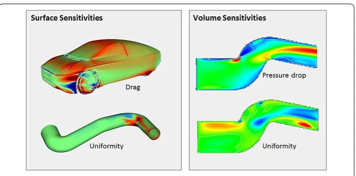
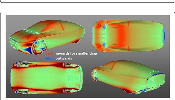
Figure 3 Sensitivity maps.Surface sensitivity maps (left) display the gradient of the cost function w.r.t. normal displacements of the surface. In red areas, a movement away from the fluid (i.e. inwards for the car, outwards for the pipe) would result in an improvement of the cost function. Contrarily, blue areas indicate the regions where a surface perturbation towards the fluid improves performance, while modifications in greenish surface sections have little effect on the cost function. The white lines on the car body are the isolines of zero sensitivity, i.e. the borderline between favourable inward and outward movement. Topological or volume sensitivities (shown on the right-hand side for a cut through the S-bend of Figure 2) represent the cost function gradient w.r.t. changes of the individual cell permeability. Blue volume sections are those where decreasing the cell permeability (by adding a porosity-based friction term) would improve the cost function. Those areas are thus counterproductive to the component’s fluid dynamic performance and should be removed - the basis of CFD topology optimisation.
w.r.t. the design variables. The computational effort is thereby independent of the number of design variables and just involves one solve of the adjoint counterparts of the govern-ing equation system, in our case the Navier-Stokes equations. When applied to a surface mesh representation or a volume mesh of the part to be optimised, information like the one depicted in Figure , for which we coined the term ‘sensitivity maps’, can be generated: A surface sensitivity map tells us for each and every surface node how the objective func-tion changes w.r.t. an infinitesimally small normal displacement of this surface node. On the other hand, a volume sensitivity map represents for each volume cell the sensitivity of the objective function w.r.t. a change of permeability of this volume cell. Both sensi-tivity maps give precise indications on where and how to change the geometry - perturb the surface inwards or outwards, and remove counterproductive cells from the flow do-main, respectively - in order to improve the objective function. Obviously, this wealth of information would be inaccessible without the adjoint method, and, as will be shown in the following, allows to develop very efficient optimisation methods for automotive part design.
Despite being already a long-established tool in the aerospace sector, the adjoint method has only recently started to also enter the automotive development processes. This backlog is mainly due to two obstacles specific to the automotive industry.
Obstacle # Rather than on in-house codes,the car industry relies almost exclusively on commercial CFD software.
adjoint) or to perform a manual or automatic differentiation of the primal code (discrete adjoint, see [] for a comparison). The sources of commercial CFD codes are, however, inaccessible for the user, and by the time we started our project to industrialise the adjoint method, the software vendors of the CFD solvers that are operational at Volkswagen de-clined to implement it into their codes. As a remedy, we selected the well-validated and versatile CFD toolbox OpenFOAM® [] as our platform to develop adjoint-based optimi-sation methods for car applications. In addition to its open source character, OpenFOAM comes with a high-level symbolic programming style, which makes it ideally suited to im-plement additional partial differential equations - like the adjoint Navier-Stokes equations. The first continuous adjoint implementation in OpenFOAM [] is based on the deriva-tion outlined in []. It focused on steady-state, incompressible ducted flows as described by the RANS (Reynolds-averaged Navier-Stokes) equations:
(v· ∇)v= –∇p+∇ ·νD(v)–αv, ()
∇ ·v= , ()
wherevandpstand for velocity and pressure, respectively, andαfor the porosity distri-bution. The effective kinematic viscosityνis the sum of molecular and turbulent viscosity, and the rate of strain tensorD(v) is defined asD(v) = (∇v+ (∇v)T). For a given cost func-tionJcomposed of contributions from the design domain boundary=∂and from the interior of,
J=
Jd+
Jd, ()
the implemented adjoint field equations are
–(v· ∇)u–∇u·v= –∇q+∇ ·νD(u)–αu–∂J
∂v, ()
∇ ·u=∂J
∂p, ()
withuandqdenoting adjoint velocity and adjoint pressure, respectively. While the cost function contribution from the domain interiorJgives rise to source terms in the adjoint field equations, the surface contributionJenters the adjoint boundary conditions:
n· ∇q= , ut= , un= –
∂J
∂p ()
for boundaries with Neumann conditions for the primal velocity and a Dirichlet condition for the primal pressure (usually inlet and wall boundaries), and
q=u·v+unvn+ν(n· ∇)un+
∂J
∂vn
, ()
=vnut+ν(n· ∇)ut+
∂J
∂vt
()
both primal and adjoint equation system, the desired (volume-normalised) topological and (surface-normalised) shape sensitivities can be computed as
∂J
∂α =u·v and ∂J
∂β = –ν∂nu·∂nv, ()
whereβdenotes the normal node displacement.
Within the still ongoing collaboration with Prof. Giannakoglou’s group at the National Technical University of Athens (NTUA) and Dr. de Villiers at Engys®, this basic implemen-tation was subsequently enhanced towards an inclusion of an adjoint turbulence model [], optimisation of external flows [], sensitivities for flow control [], adjoint wall func-tions [], the inclusion of heat conduction and constraints [] and mildly compressible flows []. In addition, the uptake and further development of the basic adjoint code by other researchers lead to remarkable advances [–], especially in the area of topology optimisation for exhaust systems [, ]. As a result of these development efforts, a ver-satile continuous adjoint code in OpenFOAM for steady-state RANS is now available.
Obstacle # The geometries of entire vehicles and even of single automotive parts are highly complex.
The complexity of typical automotive geometries, especially of entire vehicles, which consist of an assembly of several hundred parts, necessitates the use of an automatic pro-cess for the generation of the computational mesh. Even though the sophistication of au-tomatic meshing software is continuously increasing, the achievable mesh quality is still inferior to a hand-made mesh, especially concerning the creation of layers along the sur-face of the flow domain. While this quality suffices for obtaining reasonable results for pri-mal computations, it has been found that the adjoint equation system reacts much more delicately to imperfections of the computational mesh. This is particularly the case in the presence of flow separation, which is commonly encountered in flows in and around au-tomotive geometries.
This lack of robustness of the adjoint when running on typical industrial meshes is a problem that has been accompanying the adjoint development in OpenFOAM from the very beginning - and for certain applications it is still inhibiting the systematic use of the adjoint method in the regular computational processes. The source of this instability is the so-called ‘adjoint transpose convection’∇u·v- the second convection term on the left-hand side of Eqn. (). By developing several formulations for this term, as well as ex-plicit and imex-plicit treatments, major steps towards increased stability were made. As it introduces a high degree of cross-coupling between the three components of the velocity, recent efforts concentrate on solving the adjoint equation system as a single block rather than in a segregated manner [].
topology optimisation and shape optimisation for ducted flows are introduced in the next section, along with an application of these two complementary methodologies to engine port flows. Section focuses on external aerodynamics, comprising a full-vehicle vali-dation study, an example of a component optimisation and a comparison of steady-state RANS sensitivities with those based on a time-averaged transient primal flow. The article finally closes with a comparatively young adjoint application area - car drag reduction by flow control.
2 Ducted flows
Geometric optimisation of ducted flows in cars, like airducts for cabin climatisation, en-gine air intakes or exhaust systems, are commonly subject to severe packaging constraints. This gave rise to the development and adoption of topology optimisation methods for au-tomotive applications. After a concise retrospective of these development efforts, it will be shown that especially for ducted flows, topology optimisation is a perfect complement to the classical shape optimisation.
2.1 Topology optimisation
Topology optimisation is a well-established tool in computational structure mechanics [] with widespread industrial use. In its simplest realisation, a topological optimisation starts from the available design domain filled up entirely with solid material of a certain density. In an iterative fashion, the given loads are applied, the stresses are computed all over the domain and the areas with low stresses are weakened by assigning a lower density to them. After several iterations, this method retains high-density material only in regions that are critical to fulfill the structural task, and in this way generates optimal lightweight structural designs. It delivers an un-biased design from scratch that automatically fulfills the installation space constraints.
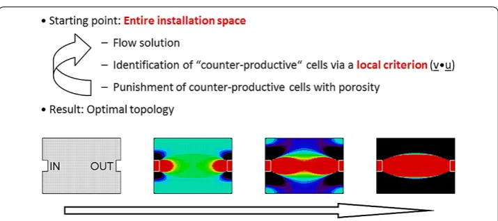
It almost comes as a surprise that it took until until this elegant concept was trans-ferred to fluid dynamics: Independently of each other Borrvall and Petersson [] and Klimetzek [] presented the first topological optimisation methods for ducted flows. Analogously to its structural mechanic archetype, their fluid dynamic topology optimi-sation starts from a completely flooded computational domain (Figure ), uses some lo-cal criterion to identify those areas that are counterproductive w.r.t. the chosen objective function and iteratively ‘punishes’ or removes them from the fluid domain. As a result, the remaining areas constitute the optimal duct between inlet(s) and outlet(s) of the given installation space.
Figure 4 The principle of CFD topology optimisation.Identified counter-productive cells are iteratively punished (black cells).
In contrast, the method proposed by Borrvall and Petersson was restricted to two-dimensional Stokes flows between parallel plates, and the punishment of counterproduc-tive areas is performed by locally decreasing the distance between the plates - until zero upon convergence. What inspired a series of subsequent research works is, however, the versatility of their approach that lies in the way how they identify counterproductive fluid cells: by computing actual sensitivities via the adjoint method.
In order to extend the Borrvall and Petersson method towards three-dimensional flows, the punishment via plate distance was replaced by introducing a Darcy porosity term –αv into the governing Eqn. () (see [] and [] for a finite-element and a finite-volume im-plementation, respectively). The individual cell porosities allow a continuous transition between fluid (α= ) and solid (α=αmax) and act as the actual design variables of the optimisation problem. With this setting, topological sensitivity maps like those shown in Figure are nothing but the derivative of the cost function w.r.t. an increase in the cell porosityα.
Another requirement for the industrial applicability of adjoint-based topology optimisa-tion was its generalisaoptimisa-tion from pure Stokes flows to turbulent Navier-Stokes flows. After the principal feasibility of laminar Navier-Stokes topology optimisation was first demon-strated via Automatic Differentiation of an academic CFD code [], the concept was implemented via a continuous adjoint also for turbulent flows [] - albeit under the as-sumption of ‘frozen turbulence’, i.e. fully neglecting the variation of the turbulent flow quantities. Finally, the development of a continuous adjoint turbulence model [] now allows to run topology optimisation for turbulent Navier-Stokes flows under full consid-eration of variations in the turbulence fields [].
As topology optimisation is not only very fast but also mimics the classical way of part design when driven by installation space constraints, the uptake of this method in the regular automotive design process was quite straightforward. A number of ducted flow applications are today routinely optimised via adjoint-based topology optimisation (see Figure for examples from the Volkswagen Group and [, ] for others). Exemplarily, one of them - the optimisation of an engine intake port - will be presented in more detail in the following.
Figure 5 Sample applications of CFD topology optimisation.Kindly provided by U Giffhorn, W Py, M Tomecki, C Ehlers, M Towara from Volkswagen AG and N. Peller from Audi AG.
Figure 6 Intake port geometry and streamlines of the original flow.Only the two arms connecting the inlet plenum and the barrel were subject to geometrical modifications upon optimising for (1) pressure drop between inlet and outlet and (2) swirl within the cylindrical slice indicated by the red mantle area.
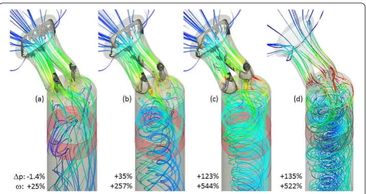
Figure 7 Intake port topology optimisation results.The three figures (a)-(c) show the Pareto-optimal states for low, mid- and high swirl weighting, respectively. The grey areas within the intake port arms are the cells that were blocked during the topology optimisation. Note the obvious improvement of swirl (ω, bottom numbers) from (a) to (c) at the cost of increasing pressure drop ( p, top numbers), as compared to the original flow of Figure 6. The topology of the high swirl case (c) was recasted into a new CAD description and recomputed (d). Flow field, swirl and pressure drop confirm the results of the topology optimisation (details see [14]).
the outlet and () to maximise the swirl, i.e. the angular momentumr×ρvaround the barrel axis in the cylindrical sub-zone indicated in Figure .
One of the main issues with multi-objective adjoint optimisation is the choice of a sen-sible relative weighting when combining the sensitivity fields from the two objectives for input into the topology update. As a first step, we therefore performed an exploration by varying the weighting factors dynamically within a wide range. After choosing three design points with different weightings (low, mid- and high swirl) that represented a likely range for desirable fluid dynamic performances of the intake port, we actually ran the topology optimisation for these three trade-offs between swirl and pressure loss until convergence and thus obtained three Pareto-optimal states (Figure a-c, details see []).
For the low swirl case, it can be assumed that the geometry is only driven by the swirl sensitivities where the modifications have a very small detrimental effect on the pressure loss. As a result, we see a small reduction in pressure loss along with a modest increase in swirl. Predictably, the pressure loss starts to go up as the swirl weighting is increased and the fluid looses additional energy due to the highly swirling flow and the blockages required to produce it. What is encouraging is the extent to which the swirl can be reliably increased - by more than % - compared to the relatively modest relative increase in pressure loss (high swirl case of Figure c).
topol-ogy optimisation run. While we do not contend that this will consistently be the case, it certainly proves the efficacy of the process in this instance.
2.2 Shape optimisation
The topology optimisation method as introduced above, acts on the fluid domain like a sculptor on a piece of rock: It removes the unwanted portions and reduces the original geometry to its optimal shape. Since the original volume mesh is not changed during the optimisation process, the final geometry consequently consists of a subset of those cells that made up the original shape. Thus, the inherent geometrical resolution of topology optimisation corresponds to the cell size, and the final shape will inevitably have a ragged surface. Topology optimisation is therefore to be regarded as adraftingmethod. For fine-tuninggeometries that are already close to their optimal shape, it is ideally complemented by so-called shape optimisation. Rather than on topological or volume sensitivities, shape optimisation is based on the detailed information contained in surface sensitivity maps in order to morph the shape towards a further improvement of the cost function.
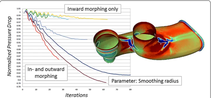
An example of a surface sensitivity map of an exhaust port is shown in Figure . Red areas are those that have to be moved outwards (away from the air) in order to reduce the pressure drop while blue regions need to be pushed inwards. It seems straightforward to translate this information into a shape modification that improves the performance of the exhaust port: Simply move every surface node in a steepest descent manner inwards or outwards by a distance corresponding to its sensitivity magnitude. Due to the inher-ent ‘roughness’ of the sensitivity distribution this would, however, quickly result in a col-lapse of the surface mesh. Therefore, a clever smoothing process has to be applied to the surface sensitivities before they are actually translated into a shape update. This smooth-ing process does not only have to generate a good compromise between ironsmooth-ing out the sharpest discontinuities of the sensitivity map and at the same time conserving the
tial sensitivity information, but also has to be capable of keeping certain feature lines of the geometry.
A surface regularisation method that comes up to these requirements has been devel-oped by Prof. Bletzinger and his team at the Technical University of Munich (TUM) [, ]. The results of applying their method to the exhaust port above are shown in Figure . Depending on the size of the smoothing radius and on whether morphing is allowed only in the inward direction or both inwards and outwards, different pressure drop reductions between % and % are achieved. Since this shape optimisation process is set up such that primal and adjoint calculation are closely coupled to the shape update itself (‘one-shot optimisation’), the overall cost of the optimisation amounts to not more than four primal computations.
As demonstrated above, topology optimisation and shape optimisation are complemen-tary methods: the former for drafting, the latter for fine-tuning. Especially for the optimi-sation of car components that are subject to design space constraints - and in the increas-ingly tighter getting installation spaces within the engine compartment and the passenger cabin this is the case for the majority of components - the combination of both meth-ods suits the requirements of automotive component design very well. Starting from the feasible installation space, they are capable of delivering a fine-tuned optimal geometry, thereby each of them making use of the full potential of the available design space.
3 External aerodynamics
The adjoint-based topology and shape optimisation methods described above are obvi-ously not restricted to ducted flows but can equally well be applied to external flows. The external aerodynamics of entire vehicles is, however, a peculiar application for optimisa-tion methods: Except for dedicated low emission cars, vehicle shapes are to a high degree driven by aesthetic considerations rather than aerodynamic performance. This has two implications: () Given the rather limited design freedom, external aerodynamic optimi-sation is more about fine-tuning. Topology optimioptimi-sation is therefore not an adequate tool. () Since aesthetic requirements can impossibly be casted into mathematical constraints, theautomaticoptimisation of vehicle shapes forbids itself - unless restricted to small por-tions like spoilers, mirrors or, of course, to the underbody.
Under these circumstances, the mere computation of surface sensitivity maps - with neither a topological nor a shape update - turned out to be a tool that fits very nicely into the specific requirements of the development of external vehicle shapes: The information contained in these maps provides the designer with concrete suggestions for aerodynamic improvements, and it is in his/her hand to translate this information into an aerodynam-ically improved shape without compromising the aesthetics.
3.1 Validation of RANS shape sensitivities for external aerodynamics
In order to validate sensitivity maps and to explore their potential for external aerodynam-ics, the adjoint method was first applied to the Volkswagen XL - a dedicated low emission vehicle developed by Volkswagen in (Figure ). Based on a steady-state RANS solu-tion on a low-Reynolds mesh of a half-model of the XL, our adjoint OpenFOAM code with adjoint turbulence model according to Zymaris et al. [] was employed to compute a sensitivity map for drag (Figure ).
Figure 9 The primal simulation for the Volkswagen XL1.The symmetry plane is coloured according to the velocity magnitude, while the car surface shows the pressure distribution.
Figure 10 Drag sensitivity maps for the XL1.Isometric front and back view, bottom view (bottom left) and top view (top right).
First of all, the ‘usual suspects’ of external car aerodynamics (the roof, the high-curvature regions of the bonnet, the areas around the wheels and the rear sillboard) are confirmed. For other sensitive areas like the spanwise blue stripe at the transition between the front-end and the bonnet (region in Figure ), it can be seen in the primal solution already that the flow detaches and requires the curvature to be reducedlocally- an adjoint is not needed to get this piece of information. The added-value of the adjoint, however, becomes obvious for regions , and : the rear end of the car where the adjoint ‘suggests’ a spoiler, the blue area of the front wing which should be further exposed, and the wheel spoiler area in front of the front tyres. This information cannot be deduced by looking only at the primal. The effect of changing the car shape here isnon-localand happens further downstream of the sensitive regions themselves. It can therefore only be identified by the adjoint.
Figure 11 Selected areas for the validation of RANS surface sensitivity maps.Rear spoiler (1), front end of bonnet (2), front wing (3) and wheel spoiler area (4).
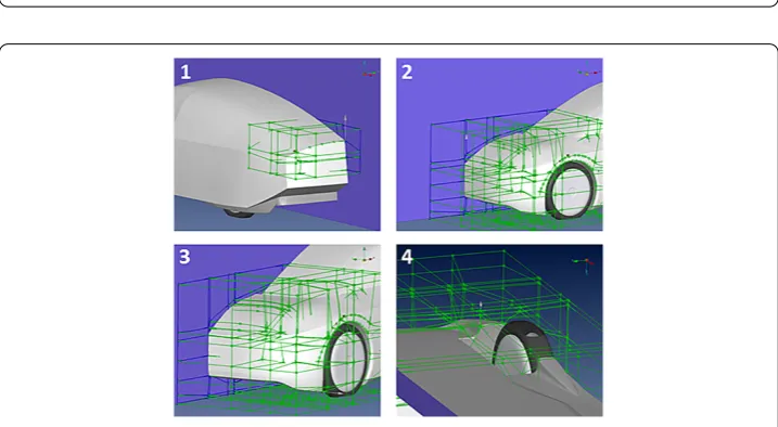
Figure 12 Definition of morphing boxes.The numbers refer to the region numbering of Figure 11 (kindly set up by BETA CAE Systems within their pre-processor ANSA®).
morphed by ‘macroscopic’ distances ( or mm, respectively) both according to and opposite to the computed sensitivity map. Recomputations of the morphed car shapes confirmed the correctness of the sensitivity signs in all cases: Morphing in the direction of the sensitivities resulted in a decrease of drag, while drag increased upon morphing opposite to the local sensitivities (Figure ). Additionally, the drag reduction resulting from a rear spoiler (region ) and from a wheel spoiler (region ) were confirmed in wind tunnel experiments.
move-Figure 13 Recomputation of morphed geometries.Given are the drag variations upon morphing in the direction suggested by the sensitivity map (left column) and in the opposite direction (right column) for a deformation by 5 or 10 mm (assumed as sensible macroscopic distances for the respective region of the car).
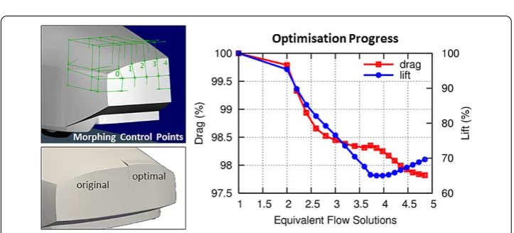
Figure 14 One-shot optimisation of the XL1 spoiler shape.The rear edge of the XL1 half-model is parameterised with five morphing control points (top left). After twenty steepest descent driven shape updates in one-shot fashion, drag reduced by 2% and lift by 30% at a total cost of five equivalent flow solutions (right). The bottom left figure compares the original and the optimal shape of the rear car edge.
ments were restricted to thez-direction (i.e. up and down, Figure ). Within a one-shot optimisation driven by a simple steepest descent algorithm thez-coordinates of the mor-phing control points were moved towards their optimal position after roughly itera-tions (Figure ). The overall cost of the optimisation corresponded to less than five pri-mal flow solutions and resulted in a drag decrease of %. Given the fact that the XL with a drag coefficient of less than . was aerodynamically nearly perfect already, this was a significant reduction. As a beneficial side-effect, lift decreased by %.
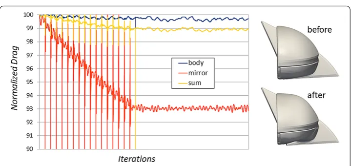
Figure 15 Shape optimisation of an external mirror.Displayed are RANS-based drag sensitivites in the mirror region of the previous Volkswagen Passat. The colouring is as usual - red regions have to be pushed inwards and blue to be pulled out in order to reduce drag.
Figure 16 Shape optimisation of an external mirror.Based on the drag sensitivities of Figure 15, the TUM morphing routines were employed to conduct a one-shot shape optimisation. Only the mirror and the triangle mounted to the car were subject to deformation. The evolution of drag on the mirrors themselves (orange curve), the remaining car body (blue) and their sum effect on the entire vehicle (yellow) are shown. Due to a missing constraint on the mirror glass area, the optimisation would ultimately generate inapplicably small mirror glasses and was therefore aborted before that happened. A constrained version of this optimisation will be published in [29]. Note how the morphing affected the overall shape of the mirror (e.g. the bulgier upstream shape and the more horizontal upper egde), but was capable of keeping the essential feature lines of the original design. An illustrative movie of the shape evolution during optimisation is provided asAdditional file1.
and every node into its optimal position, they are ideally suited for the optimisation of vehicle details - like external mirrors.
Figure 17 The current Audi A7.As simplifications for the primal flow model, the engine bay was completely sealed (i.e. no underhood flow) and the floor was assumed stationary.
3.2 RANS sensitivities vs. approximate time-averaged DES sensitivities
The preceding section summarised the achievements in the development of adjoint-based shape optimisation methods for external aerodynamics of vehicles. These methods rest upon steady-state RANS simulations. Meanwhile, however, the common practice of ex-ternal aerodynamics computations has moved - at least in the largest part of the Volkswa-gen Group - from steady-state RANS to unsteady Detached-Eddy Simulations (DES, []). To create an adjoint to a time-varying primal like DES entails particular difficulties: Since the adjoint runs backwards in time, all primal states for the time period of interest have either to be stored or recomputed when running the adjoint. The huge amount of storage space and computational time can, in principle, be reduced to a manageable amount by clever checkpointing algorithms [, ], but for the typical model sizes of car external aerodynamics an adjoint to a DES run is still not feasible yet.
Our provisional solution to compute sensitivity maps for primal DES computations therefore looks as follows: We plug the time-averaged velocityvand pressurepfrom the primal DES computation into a RANS turbulence model in order to solve for a turbulent viscosityνt. With these quantities - time-averagedvandpas well as RANS-νt - we run the existing RANS adjoint code to obtain the sensitivities. A validation study similar to the one above for the XL revealed that we can only expect qualitative accuracy from this procedure. Quantitatively, the sensitivities are not correct. Still, the following comparison will demonstrate that these approximate DES sensitivities are useful and actually have an added value against pure RANS sensitivities.
Figure 18 RANS vs. approximate DES sensitivities.Note the similarity between RANS- and DES-based drag sensitivities for the largest part of the car hat - and the dramatic difference at the rear part. While the RANS computation misses the favourable effect of a rear spoiler, it is clearly present in the DES results.
Figure 19 RANS vs. approximate DES sensitivities.A rear view of the sensitivity differences in the spoiler area, and the actual shape of the active spoiler in the current Audi A7.
clearly present in the DES counterpart. It is this kind of results that - despite the lack of their quantitative accuracy - gave a lot of credibility to our provisional solution of com-puting sensitivities based on DES primals and supported their integration into the regular computational processes for external aerodynamics (see Figure ).
3.3 Adjoint methods for flow control
Figure 20 RANS vs. approximate DES sensitivities.The RANS-based sensitivities also fail to predict the beneficial effect of further lateral tapering of the car’s back (‘boat-tailing’).
Figure 21 Drag sensitivity maps based on DES.Further examples of drag sensitivity maps for various car models of Volkswagen and Audi as computed by the outlined DES-based method.
on drag and lift, while Heinemann et al. [] experimentally investigated continuous jets on a : model of a passenger production car.
Since flow control of entire vehicles is a rather young subject, experience for the opti-mal layout of jet configurations is still very limited. The questions to be answered when designing a flow control concept are: () What kind of jets should be applied - blowing or suction? () Where should the jets be positioned to have a maximum effect? () What is the achievable aerodynamic improvement?
Figure 22 Flow control sensitivities for the Ahmed body.Based on a RANS computation, a flow control sensitivity map of dragFxw.r.t. normal jet velocityvnwas computed for the 35◦case of the Ahmed body. The
highest sensitivities are expectedly encountered at the rear part. Suction is favourable at the rear separation edge and at the origin of the longitudinal vortices, whereas on the slant surface blowing would reduce the drag by filling the wake.
mass flux through it, and the adjoint method is then applied to compute the sensitivity of dragFxor liftFzw.r.t. changing the mass flux through each of the ‘holes’ [].
Figure shows such a sensitivity map for the Ahmed body, i.e. the distribution of
∂Fx/∂vn. Blue areas are those where blowing (vn> ) would result in drag reduction, while in red areas a suction jet would help to reduce drag. The colour intensity indicates the mag-nitude of the effect on the dragFx. The computation was carried out on a low-Reynolds mesh (y+≈) using a RANS primal with the Spalart-Allmaras turbulence model and its adjoint counterpart.
The validation of these sensitivities is shown in Figure . At two different locations, one in the blue and another in the red region, various normal velocities ranging from – m/s (suction) to + m/s (blowing) were applied in order to compute their effect on drag. As expected, for small jet velocities of up to m/s, the sensitivity captures the gradient Fx/ vnvery well. But surprisingly, still for higher jet velocities the sensitivity constitutes a good approximation to the actual effect of the jet. In conclusion, flow control sensitivity maps do not only indicate whether a suction jet or a blowing jet is favourable and where to place it, but also give a useful estimate of the achievable effect.
Figure 23 Flow control sensitivities for the Ahmed body.For validation purposes, normal jet velocities between –40 m/s (suction) and +40 m/s (blowing) were applied on surface elements at two different locations of opposite sensitivity signs (pink and yellow spot, respectively). The blue squares indicate the computed drag values, and the red lines correspond to the sensitivity of the respective locations. Note the qualitative and quantitative agreement even for high jet velocities.
Figure 25 Wind tunnel measurements of the XL1.In addition to force measurements and oil film visualisation, PIV measurements were conducted in four different planes in the car’s wake, including the symmetry plane (data kindly provided by R Petzold and P Scholz from the Technical University of Braunschweig [38]).
Figure 26 PIV measurements in the symmetry plane of the XL1 wake.Note the slightly smaller recirculation area and the upwardly directed flow when the jets are switched on (see [38] for details).
corners of the car (Figure ). As a result, lift dropped by %, and drag - in accordance with the computed sensitivities - decreased by about %. Even though this additional drag reduction of % is significant for a car like the XL, it is unfortunately not enough to in-corporate a jet system into a car and run it productively.
4 Summary and outlook
pro-Figure 27 PIV measurements in a perpendicular plane behind the XL1.Upon switching on the jets, the two counter-rotating longitudinal vortices are effectively weakened. This goes along with less downwash and hence decreased lift (see [38] for details).
cess has just started with some initial promising results. Both methods will most surely have an impact on overall vehicle performance and consumption in the future.
The adjoint development efforts have so far concentrated on steady-state phenomena. For an extension towards inherently transient flow applications, like aeroacoustics, flow control with pulsating jets and transient aerodynamics with DES, the adjoint has to be-come transient as well. This is a subject that is under investigation by several research groups already (e.g. [–]) and is currently addressed in the Marie-Curie International Training Network ‘aboutFlow’ []. Its industrialisation can be regarded as the next chal-lenge in developing adjoint methods for the automotive industry.
Additional material
Additional file 1: External mirror shape optimisation.How the shape of the external mirror of Figures 15 and 16 evolves from the original to the optimal shape and back again is illustrated by this movie. The colour represents the magnitude of node displacement as compared to the original (details see [28, 29]).
Competing interests
The author declares that they have no competing interests.
Acknowledgements
The author is truly grateful to E de Villiers and his colleagues at Engys, KC Giannakoglou and his team at NTUA (above all EM Papoutsis-Kiachagias and AS Zymaris), E Stavropoulou, M Hojjat and KU Bletzinger from TUM, JD Müller (Queen Mary University London) and the FlowHead team, as well as E Skaperdas and K Haliskos from BETA CAE Systems. The support from many CFD colleagues of the Volkswagen Group in the form of continuous interest in the adjoint method, provision of resources and of valuable feedback is also gratefully acknowledged.
Received: 30 March 2013 Accepted: 5 March 2014 Published: 3 June 2014
References
1. Lions JL:Optimal Control of Systems Governed by Partial Differential Equations. New York: Springer; 1971. 2. Pironneau O:On optimum design in fluid mechanics.J Fluid Mech1974,64:97-110.
3. Jameson A:Aerodynamic design via control theory.J Sci Comput1988,3:233-260.
4. Löhner R, Soto O, Yang C:An adjoint-based design methodology for CFD optimization problems.AIAA-03-0299
2003.
5. Nadarajah S, Jameson A:A comparison of the continuous and discrete adjoint approach to automatic aerodynamic optimization.AIAA-00-06672000.
6. OpenFOAM®- The Open Source CFD Toolbox[http://www.openfoam.com]
7. Othmer C, de Villiers E, Weller HG:Implementation of a continuous adjoint for topology optimization of ducted flows.AIAA-2007-39472007.
8. Othmer C:A continuous adjoint formulation for the computation of topological and surface sensitivities of ducted flows.Int J Numer Methods Fluids2008,58:861-877.
9. Zymaris AS, Papadimitriou DI, Giannakoglou KC, Othmer C:Continuous adjoint approach to the Spalart-Allmaras turbulence model for incompressible flows.Comput Fluids2009,38(8):1528-1538.
10. Othmer C, Papoutsis-Kiachagias EM, Haliskos K:CFD optimization via sensitivity-based shape morphing. In
11. Zymaris AS, Papadimitriou DI, Giannakoglou KC, Othmer C:Optimal location of suction or blowing jets using the continuous adjoint approach. InProceedings of the 5th European Conf. on Computational Fluid Dynamics, Lisbon, Portugal, ECCOMAS CFD2010.
12. Zymaris AS, Papadimitriou DI, Giannakoglou KC, Othmer C:Adjoint wall functions: a new concept for use in aerodynamic shape optimization.J Comput Phys2010,229(13):5228-5245.
13. Kontoleontos EA, Papoutsis-Kiachagias EM, Zymaris AS, Papadimitriou DI, Giannakoglou KC:Adjoint-based constrained topology optimization for viscous flows, including heat transfer.Eng Optim2013,45(8):941-961. 14. de Villiers E, Othmer C:Multi-objective adjoint optimization of intake port geometry.SAE Technical Paper
2012-01-09052012.
15. Helgason E, Krajnovic S:Aerodynamic shape optimization of a pipe using the adjoint method. InProceedings of the ASME 2012 International Mechanical Engineering Congress & Exposition, Houston, Texas, USA, IMECE2012.
16. Lincke A, Rung T:Adjoint-based sensitivity analysis for Buoyancy-driven incompressible Navier-Stokes equations with heat transfer. InProceedings of the Eighth Internat. Conf. on Engineering Computational Technology, Dubrovnik, Croatia2012.
17. Jakubek D, Wagner C:Shape optimization of train head cars using adjoint-based computational fluid dynamics. InProceedings of the First International Conference on Railway Technology, Las Palmas de Gran Canaria, Spain2012. 18. Towara M:Numerical optimization of an oil intake duct with adjoint topological methods.Diploma thesis. RWTH
Aachen University, Dept. of Software and Tools for Computational Engineering; 2011.
19. Hinterberger C, Olesen M:Automatic geometry optimization of exhaust systems based on sensitivities computed by a continuous adjoint CFD method in OpenFOAM.SAE Technical Paper 2010-01-12782010.
20. Hinterberger C, Olesen M:Industrial application of continuous adjoint flow solvers for the optimization of automotive exhaust systems. InProceedings of the ECCOMAS Thematic Conf. - CFD & Optimization, Antalya, Turkey, ECCOMAS2011.
21. Giannakoglou KC:Continuous adjoint methods in shape, topology, flow-control and robust optimization. InOpen Source CFD International Conference, London, UK, ICON-CFD2012.
22. Bendsoe MP, Sigmund O:Topology Optimization: Theory, Methods and Applications. Berlin: Springer; 2004. 23. Borrvall T, Petersson J:Topology optimization of fluids in Stokes flow.Int J Numer Methods Fluids2003,41:77-107. 24. Moos O, Klimetzek F, Rossmann R:Bionic optimization of air-guiding systems.SAE Technical Paper 2004-01-1377
2004.
25. Gersborg-Hansen A, Sigmund O, Haber R:Topology optimization of channel flow problems.Struct Multidiscip Optim2005,30:181-192.
26. Othmer C, Grahs T:Approaches to fluid dynamic optimization in the car development process. InProceedings of the EUROGEN Conference, Munich, Germany2005.
27. Othmer C, Kaminski T, Giering R:Computation of topological sensitivities in fluid dynamics: cost function versatility. InProceedings of the ECCOMAS CFD Conference, Delft, The Netherlands2006.
28. Stavropoulou E, Hojjat M, Bletzinger KU:In-plane mesh regularization for node-based shape optimization problems.Comput Methods Appl Mech Eng, in press
[http://www.sciencedirect.com/science/article/pii/S004578251400070X]
29. Hojjat M, Stavropoulou E, Bletzinger KU:The vertex morphing method for node-based shape optimization.
Comput Methods Appl Mech Eng2014,268:494-513.
30. ANSA®pre-processor – BETA CAE Systems S.A.[http://www.beta-cae.gr/ansa.htm]
31. Islam M, Decker F, de Villiers E, Jackson A, Gines J, Grahs T, Gitt-Gehrke A, Comas i Font J:Application of detached-Eddy simulation for automotive aerodynamics development.SAE Technical Paper 2009-01-03332009. 32. Griewank A:Achieving logarithmic growth of temporal and spatial complexity in reverse automatic
differentiation.Optim Methods Softw1992,1:33-54.
33. Wang Q, Moin P, Iaccarino G:Minimal repetition dynamic checkpointing algorithm for unsteady adjoint calculation.SIAM J Sci Comput2009,31(4):2549-2567.
34. Brunn A, Wassen E, Sperber D, Nitsche W, Thiele F:Active drag control for a generic car model.Notes Numer Fluid Mech Multidiscipl Des2007,95:247-259.
35. Ahmed SR, Ramm R, Falting G:Some salient features of the time-averaged ground vehicle wake.SAE Technical Paper 84-03001984.
36. Bideaux E, Bobillier P, Fournier E, Gillieron P, El Hajem M, Champagne JY, Gilotte P, Kourta A:Drag reduction by pulsed jets on strongly unstructured wake: towards the square back control.Int J Aerodyn2011,1(3/4):282-298. 37. Heinemann T, Springer M, Lienhart H, Kniesburges S, Becker S:Active flow control on a 1:4 car model. InProceedings
of the 16th Int. Symp. on Applications of Laser Techniques to Fluid Mechanics, Lisbon, Portugal2012.
38. Petzold R:Experimentelle Untersuchungen zur Strömungsbeeinflussung an einem 1:4-Fahrzeugmodell.Diploma thesis. TU Braunschweig, Inst. für Strömungsmechanik; 2011.
39. Torbert S, Löhner R:Checkpointing schemes for adjoint methods and strongly unsteady flow.AIAA-2012-0572
2012.
40. Economon TD, Palacios F, Alonso JJ:A coupled-adjoint method for aerodynamic and aeroacoustic optimization.
AIAA-2012-55982012.
41. Carnarius A, Thiele F, Özkaya E, Nemili A, Gauger N:Optimal control of unsteady flows using a discrete and a continuous adjoint approach. InProceedings of the 25th Conference on System Modeling and Optimization, Berlin, Germany; 2011:318-327.
42. aboutFlow - Adjoint-based optimisation of industrial and unsteady flows[http://aboutflow.sems.qmul.ac.uk]
doi:10.1186/2190-5983-4-6