R E S E A R C H
Open Access
Reversible audio data hiding algorithm
using noncausal prediction of alterable
orders
Shijun Xiang
1,2*and Zihao Li
1Abstract
This paper presents a reversible data hiding scheme for digital audio by using noncausal prediction of alterable orders. Firstly, the samples in a host signal are divided into thecrossand thedotsets. Then, each sample in a set is estimated by using the pastPsamples and the futureQsamples as prediction context. The orderP + Qand the prediction coefficients are computed by referring to the minimum error power method. With the proposed predictor, the prediction errors can be efficiently reduced for different types of audio files. Comparing with the existing several state-of-the-art schemes, the proposed prediction model with expansion embedding technique
introduces less embedding distortion for the same embedding capacity. The experiments on the standard audio files verify the effectiveness of the proposed method.
Keywords:Reversible data hiding, Audio, Noncausal prediction, Minimum error power, Alterable orders
1 Introduction
Reversible data hiding technique is used for embedding data in a host signal and the host signal can be com-pletely recovered [1]. It is used for keeping host signal such as medical images and audio files losslessly. There are two significant criterions for reversible data hiding techniques: the embedding capacity should be large while the distortion should be low. These two criterions conflict with each other. Usually, a higher embedding capacity is accompanied by a higher distortion.
Early reversible data hiding algorithms mainly focused on lossless compression. To embed data into a host signal, vacant space was made by compressing a part or even the whole host signal. Fridrich et al.proposed reversible data hiding algorithms using compression of bitplane [2] and vector state [3] for better performance. In [4], Celik et al. proposed a lossless generalized-LSB data hiding method which compressed a set of selected features from an image and embedded the payload in the space made by the compression. The type of methods usually achieved a low capacity with severe distortion.
For improving data hiding performance, Tian in [5] in-troduced a difference expansion (DE)-based method, in which every two pixels were grouped together to produce one high-pass coefficient and one low-pass coefficient. Then, a high-pass coefficient should be expanded to carry 1 bit. That is to say, two pixels were used to embed 1 bit. To solve the overflow and underflow problems, a location map should be used to mark the out of range pixels and embed together with the payload. Therefore, the embed-ding capacity is at best 0.5 bit/pixel. Tian’s method is a fundamental work of reversible data hiding and has been developed in many aspects, such as Alattar’s technique which embedded two data bits in every three pixels [6], the reduction of the size of location map [7] and the strat-egy to generalize DE into integer transform [8, 9].
Another type of improvement called prediction error expansion (PEE) has exceeded the DE-based methods. In these schemes, pixels were first predicted by their con-texts, and the prediction error was used for data embed-ding through expansion. The superiority of PEE is that it can better explore the correlation to improve the predic-tion performance and reduce the embedding distorpredic-tion. In [10], Thodi and Rodriguez proposed a histogram shifting method for embedding data in prediction errors. This paper established the foundation of PEE. Then, the
* Correspondence:[email protected]
1School of Information Science and Technology, Jinan University, Guangzhou 510632, China
2State Key Laboratory of Information Security, Institute of Information Engineering, Chinese Academy of Sciences, Beijing 100093, China
two authors also proposed an improvement’s method based on difference expansion technique [11]. There are many different predictors for PEE, such as partial differ-ence expanding (PDE) predictor [12], edge-detection mechanism (MED) [13] predictor, Gaussian weight pre-dictor [14], or accurate prepre-dictor [15].
On the basis of DE and PEE, histogram shifting (HS) technique has been developed. HS-based scheme was first proposed by Ni et al. [16]. The significant part of the scheme was to shift the right and left bins of the peak fre-quency bin to make room for data embedding. Thus, the number of the peak frequency bin determines the embed-ding capacity. These schemes may include blocking or area selection methods just like the approach shown in [17]. Its embedding capacity was usually smaller and the embedding distortion was unstable. For bigger capacity and lower distortion, some works have combined PE with HS, such as the reference [18]. A sharper prediction-error histogram can be obtained from PE while HS can reduce embedding distortion.
For better prediction performance, Yan and Wang pro-posed a prediction-error expansion method using linear prediction [19] which used past eight samples for predic-tion and the predicpredic-tion coefficients were integers and the order was fixed. In [20], Nishimura combined linear prediction method and error expansion technique that the past eight samples used to compute prediction coef-ficients. For exploring the correlation of the neighbor pixels/samples adequately, in [21], a non-integer predic-tion error expansion embedding method was proposed. In this method, the prediction value of the current sam-ple was the mean of its two closest samsam-ples. Sachnev et al. [22] proposed a double-embedding scheme, which separated an image into two sets so that the pixels can be predicted with four immediate pixels. Hu et al. [23] presented an image data hiding scheme by using mini-mum rate prediction and optimized histogram modifica-tion method.
There is still room for improvement in these PEE-based excellent works by using better prediction method with different order for different clips. In this paper, the PEE technique is further explored and a new reversible audio data hiding scheme is presented with two improve-ments to PEE:
1) Noncausal predictor. Due to conventional predictors of PEE which the prediction coefficients keep unchanged [19,21,22] or only past samples (or pixels) are used as prediction context, the redundancy can not be explored effectively [19,20]. To answer this question, we proposed a new noncausal predictor by combining the advantages of linear predictor and conventional noncausal predictor. This predictor is designed for the double-embedding scheme in which
the prediction coefficients can be adaptively calculated by minimum error power method.
2) Alterable orders. Unlike conventional predictors of PEE which the prediction order is fixed [19–23] and where the prediction errors can not be effectively reduced for different audio files, the noncausal linear predictor with alterable orders is proposed in this paper. The optimal prediction order can be chosen according to the complexity of an audio file by using minimum error power method.
Owing to our improvements, the sharper prediction-error histogram can be obtained for the reduction of embedding distortion. With several standard clips, ex-perimental results have shown that the prediction orders are different for different clips, and the best prediction performance can be achieved for a candidate file. Compar-ing with existCompar-ing reversible audio data hidCompar-ing methods, the proposed one has lower distortion at the same embedding rate.
The rest of the paper is organized as follows: the pro-posed scheme is described in Section II, and the experi-mental results in comparison with several existing excellent methods are reported in Section III. The Conclusions is in the last section.
2 The proposed scheme
This section presents the proposed noncausal prediction model in detail, which can provide satisfactory prediction accuracy for different clips. The double-embedding strat-egy [22] is introduced for the proposed prediction model to form the proposed high-capacity reversible data hiding scheme.
2.1 Double-embedding strategy
The double-embedding strategy has been proposed for reversible image data hiding in [22] by dividing an image into two sets like a chess board. In such a way, the pixels in a set can be predicted with its four immediate pixels in the other set. In the encoder, the first set was marked at first. In the decoder, the second set was recovered at first.
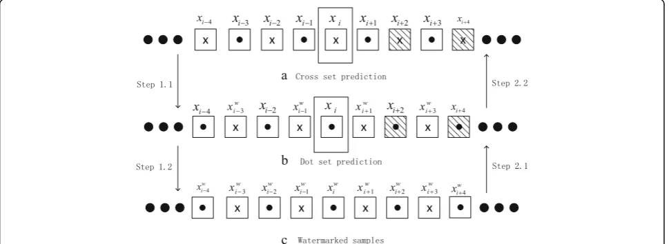
In this paper, an audio sequence is divided into two sets: cross set and dot set, as shown in Fig. 1. The samples in the cross set are predicted for expansion embedding at first. The detailed embedding and extraction operations are described in part E and part F of Section II.
2.2 Noncausal prediction model
In the proposed prediction model, a sample is estimated
by using the linear combinations of its P past samples
andQfuture samples as prediction context. This is more efficient to reduce the prediction error than only using
the past samples as prediction context. The prediction valuexiof the current samplexiis given by:
xi¼round XP
k¼1
akxi−kþ XQ
k¼1
aPþkxiþ2k−1 !
ð1Þ
Where P and Qare integers, and ak(k= 1, 2,…,P+Q) are the prediction coefficients. K=P+Q is defined as the order of the prediction model in this paper.
2.3 Estimate of prediction coefficients
Before the prediction step, we use a sorting model to sort the distances of the current sample and those neigh-boring samples (the past 40 samples and the future 20 samples). First, we calculate the distance between the current sample and the neighboring samples as
dPp¼ XL−Q
i¼
d
P2
e
x2iþ1−x2iþ1−p
dQq¼ XL−Q
i¼
d
P2
e
x2iþ1−x2iþ2q
8 > > > > > > > > > > < > > > > > > > > > > :
ð2Þ
where dPp(p= 1, 2,…,P) is the distance between the current sample and the pastpsamples whiledQq(q= 1,
2,…,Q) is the distance between the current sample and
the future 2q−1 samples, L is the number of the
sam-ples in the cross or the dot set. And L¼N
2 where Nis
the length of the audio file.
After the distances have been calculated, we propose a sorting method to sort the distances. For example, if dP1<dQ1<dP3<dP2<dQ2 and the optimal K is 3, we
letP= 2 andQ= 1. For eachi, we usexi−1,xi−3andxi+ 1
to calculate the prediction coefficients. For better expres-sion, we denotexP1
i asxi−1,xPi2 asxi−3,xPi3 asxi−2,xQi1 as
xi+ 1andxQi2 asxi+ 3. In other words, we usexPi1,xPi2 and
xQ1
i for prediction.
For the sorting method, we modify the Eq. (1) as
xi¼round XP
k¼1 akxPikþ
XQ
k¼1 aPþkxQik
!
ð3Þ
For the current sample xi, we denote the sample set
UKi as its prediction context and the setAKas its predic-tion coefficients, formulated as follows:
UiK¼ xP1i ;xP2i ;⋯;xiPP;xQ1i ;xQ2i ;⋯;x QQ
i
h iT
ð4Þ
and
AK ¼ a
1;a2;⋯;aP;aPþ1;aPþ2;⋯;aPþQ
ð5Þ
WhereTis the transposition operation on a matrix. Fig. 1Audio sequence represented ascrossanddotsets
In this paper, we propose to use minimum error power method [24] to estimate the prediction coefficients by
computing the minimum error power. For a given K
value, the error power value ρK in the cross or dot set can be computed as
ρK ¼ 1
L−2dP 2e−Q
XL−Q
i¼dP
2e
x2iþ1− AK TUK2iþ1
h i2
ð6Þ
Referring to (3), there are 2P
2þQ samples not
predicted for the computation.
From (6), we can compute the prediction coefficients AKby minimizingρK. This can be done by the following formulation,
dρK
dAK¼0 ð7Þ
From (6) and (7), we have the following deduction,
2 L−2dP
2e−Q XL−Q
i¼dP
2e
x2iþ1− AK TUK2iþ1
h i
UK2iþ1
T
¼0
Fig. 3Framework of the double embedding and extracting scheme
Fig. 4Different K1for 4 example clips of the cross set prediction and the error power results
⇒XL−Q i¼dP
2e
UK2iþ1 x2iþ1− UK2iþ1
T
AK
h i
¼0
⇒ XL−Q i¼dP
2e UK
2iþ1 UK2iþ1
T
AK ¼X
L−Q
i¼dP 2e
x2iþ1UK2iþ1 2
4
ð8Þ
From (8), the prediction coefficient set AK can be
computed by the following expression,
⇒AK¼ X
L−Q
i¼dP
2e
UK2iþ1 UK2iþ1
T
2 4
3 5 −1
XL−Q
i¼dP
2e
x2iþ1UK2iþ1
ð9Þ
Fig. 5Different K2in different T1for clip 39 of the Cross set prediction and the error power results
After the prediction coefficients AK are estimated, the
minimum error power value with the order K can be
computed by referring to (6).
2.4 The prediction order
How to compute the prediction orderKis a crucial step
since it plays an important role for the reduction of the prediction errors. Too small a size can not effectively
explore the correlation among samples, and too large a size will bring negative effects since a sample not close to the current sample has less correlation. For different
audio files, the order K may be different in order to
achieve an ideal prediction accuracy. In Section II-C, we
have shown that for a given orderK, the minimum error
power ρK and the corresponding coefficient set AK can
be computed for the prediction. For different order Fig. 7Different K2in different T1for clip 64 of thecrossset prediction and the error power results
Fig. 8Different K2in different T1for clip 66 of thecrossset prediction and the error power results
values, we can get different minimum error power values. Among all the minimum error power values, the smallest one is corresponding to the order and the pre-diction coefficients used for reversible data hiding.
For better description, in this work we denoteK1and
K2 as the orders of the prediction coefficients in the
cross set and dot set, respectively. Let AK1 be the pre-diction coefficients for the cross set while AK2 for the dot set.
2.5 Data embedding and extraction methods
After the prediction, expansion embedding combined with histogram shifting techniques proposed in [10] are applied to hide information bits reversibly. A threshold
valueT is defined by referring to the embedding
cap-acity. The prediction errors in the range [−T,T] will be expanded to carry the data bits while those not in [−T,T] are shifted to make room for the expansion.
In the encoder, the samples in the cross set are pre-dicted and watermarked at first. Suppose the prediction value of the current sample xiis xi, the prediction error
eiis calculated as
ei¼xi−xi ð10Þ
Then, the information bits can be inserted by the fol-lowing rules:
Di¼
2eiþb; eiþT þ1;
ei−T; if if if 8
< :
ei∈ −½ T;T ei>T ei<−T
ð11Þ
Where Di is the prediction error after expansion
em-bedding and b is a bit to be hidden. After the
embed-ding, the samplexiis watermarked as
xwi ¼xiþDi ð12Þ
Once the watermark embedding operations on the samples in the cross set have been finished, the similar embedding process will be implemented on the samples in the dot set. Figure 2 shows prediction, watermark em-bedding, and watermark extraction processes of the cross set and the dot set. In Fig. 2a, the original samples (unshadowed) are used to predict the cross set, and then watermark bits are embedded into the cross set in Step 1.1. After that, the dot set samples are predicted by ori-ginal dot oriori-ginal samples and watermarked cross sam-ples, and the watermark bits are inserted into the dot set in Step 1.2.
In the decoder, we extract the hidden bits from the dot set and recover the samples in this set at first. For
the sample xi, the sample prediction operation can be
used to obtainxi. Then we have
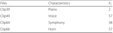
Table 1The orders (K1) for 4 different clips
Files Characteristics K1
Clip39 Piano 2
Clip49 Voice 57
Clip64 Symphony 38
Clip66 Horn 57
Fig. 10Histograms of the prediction errors with four different predictors for clip 39
Fig. 11Histograms of the prediction errors with four different predictors for clip 49
Fig. 12Histograms of the prediction errors with four different predictors for clip 64
Di¼xwi−xi ð13Þ
The hidden information bit is extracted and the original sample is recovered as
b¼Dimod2;Di∈ −½ 2T;2Tþ1 ð14Þ
and
ei¼
floor Di 2 ; Di−T−1;
DiþT; 8
> > < > > :
if if if
Di∈ −½ 2T;2Tþ1 Di>2Tþ1
Di<−2T
ð15Þ
and Fig. 14SNR comparison of the proposed scheme against three typical methods for clip 39
Fig. 15SNR comparison of the proposed scheme against three typical methods for clip 49
xi¼xiþei ð16Þ
Once the decoding operations on the samples in the dot set have been finished, the similar extraction process is implemented on the samples in the cross set. As shown in Step 2.1 in Fig. 2, we first recover the original samples of the cross set and extract the payload. Then the original samples of the dot set are recovered and the payload is
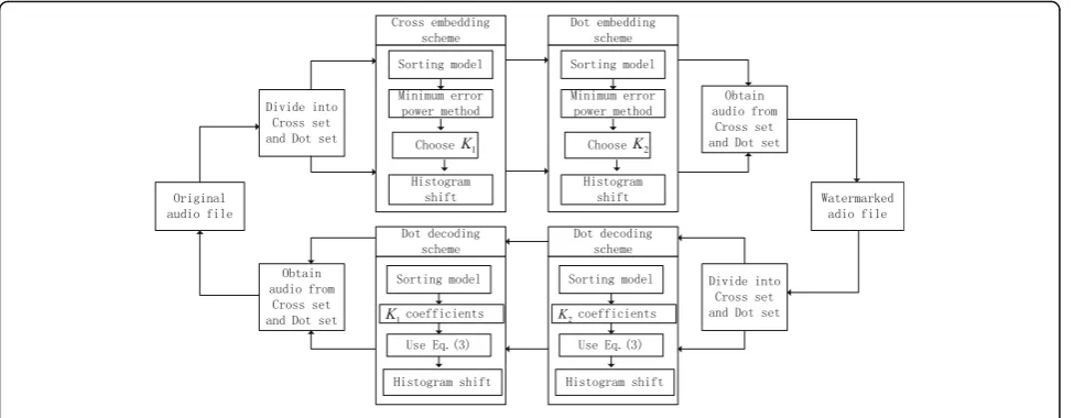
extracted completely by Step 2.2. The sketch of the pro-posed watermarking scheme is shown in Fig. 3.
2.6 Auxiliary information
In the proposed scheme, the auxiliary information in-cludes the threshold values (T1 for the cross set andT2
for the dot set), the prediction orders (K1=P1+Q1and
K2=P2+Q2), and the prediction coefficients (AK1 and
Fig. 16SNR comparison of the proposed scheme against three typical methods for clip 64
AK2). The auxiliary information should be inserted into the cover signal for blind extraction.
In experimental way, the size of the auxiliary informa-tion is assigned as follows:
1. In the testing, all the samples can be used for reversible data hiding when the threshold value is bigger than 800. So, we use 20 bits to reserve
the threshold valuesT1(10 bits) andT2 (10 bits)
since 10 binary bits can represent 1024 at most. 2. We use 12 bits to reserve the values ofK1(6 bits) andK2
(6 bits). The basic reason is that in the testing the threshold value is always smaller than 64 for all the clips. 3. In our testing, the prediction coefficients in
magnitude are always smaller than 10. For a trade-off between prediction accuracy and embedding
Fig. 18ODG comparison of the proposed scheme against three typical methods for clip 39
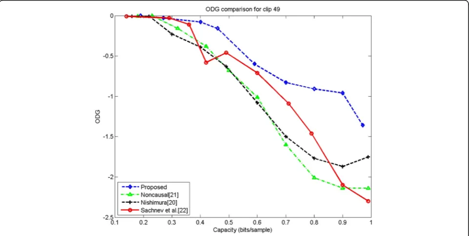
Fig. 19ODG comparison of the proposed scheme against three typical methods for clip 49
efficiency, all the coefficients only keep two decimal places by using rounding operation. For example, when the prediction coefficienta1 is 1.4433, it will be rounded to 1.44; whena2 is−0.3852, it is rounded to−0.39. After expanding one hundred times, we can use 11 bits to represent a coefficient (10 bits for the magnitude, 1 bit for the sign).
4. In the embedding, the underflow and overflow problems have been considered by using location map. For a sample with the underflow or overflow problem, we use 25 bits to mark its position since most of the clips (44.1 kHz in duration) are not longer than 12 min. Due to the fact that the proposed prediction model has higher accuracy,
Fig. 20ODG comparison of the proposed scheme against three typical methods for clip 64
there are lesser samples with the underflow and overflow problems by testing all example clips. 5. Considering the auxiliary information above, in our
scheme we use 12 bits to save the length of the auxiliary information, which can indicate 4096 bit of auxiliary information at most.
In the encoder, the LSB values of the firstM+ 12 sam-ples are saved as part of the payload to reversibly embed into the cover signal. Here,Mis the length of the auxil-iary information. We use the LSB positions of the first 12 samples to record the length. Then the LSB positions
of the next M samples are used to keep the auxiliary
Fig. 22
Fig. 23ODG comparison of the proposed scheme against three typical methods for 70 audio clips
information. In the decoder, the auxiliary information is
first extracted from the LSB values of the first M+ 12
samples for the extraction of the hidden bits and the re-covery of the cover signal.
3 Experimental results
In reversible data hiding community, embedding rate and distortion are two significant criterions. In the testing, we use signal to noise ratio (SNR) and PEAQ software to choose objective difference grade (ODG) to measure the watermark distortion of reversible data hiding schemes. The bit per sample (bps) is adopted to measure the em-bedding rate. The test data set includes 70 standard audio files (the wave format with the sampling rate of 44.1 kHz) [25]. Here, four clips marked by 39, 49, 64, and 66 are ran-domly selected as example clips for report.
Figure 4 shows the differentK1(the cross set prediction
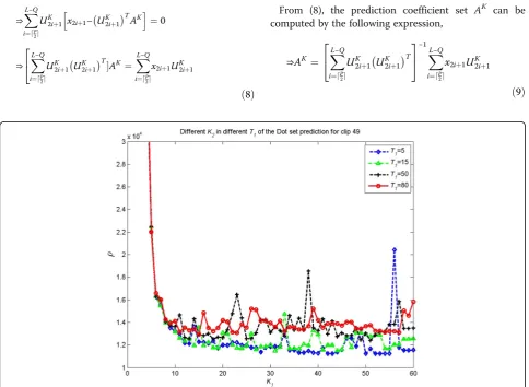
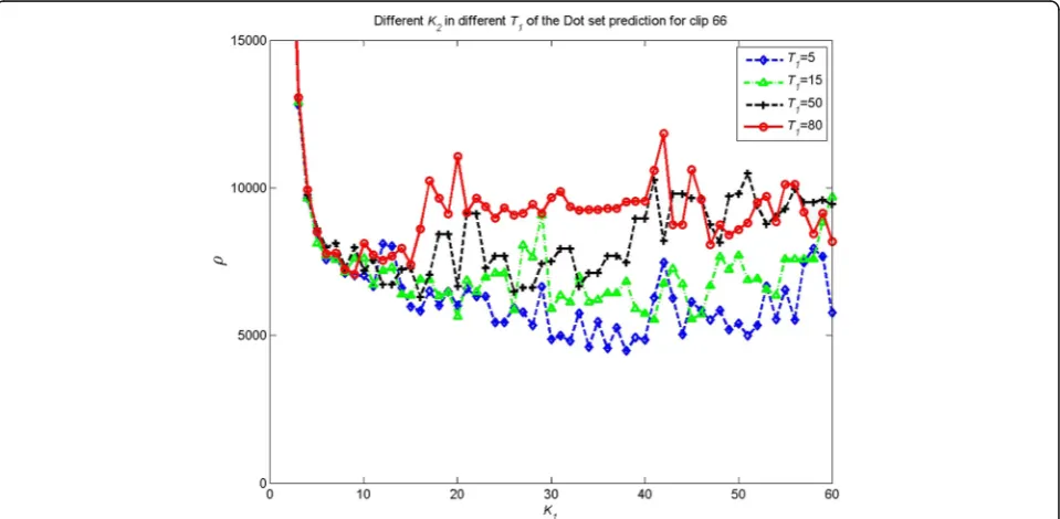
order) and error power values for 4 example clips. We can see that different audio clip have differentK1. Figures 5, 6,
7, and 8 show the different K2 (the dot set prediction
order) for 6 audio clips with two thresholds 5 and 15 in case of low capacity while with two thresholds 50 and 80 in case of high capacity. We also observe that for the same clip, the orderK2is often different fromK1. TheK2value
mainly depends onK1and the low capacity thresholds (5
and 15). In other words, the largerK1and the lower
cap-acity thresholds, the largerK2. The basic reason is thatK1
is estimated by using the original samples but K2is not.
After the cross set is watermarked, the embedding distor-tion has an effect on the computadistor-tion ofK2.
Table 1 shows the four different types of example clips. For each clip, the order of the prediction coefficients for the cross setK1is computed and listed. We can see that
different types of audio files have different optimal pre-diction orders. For all the 70 audio clips, we show their optimalK1values in Fig. 9.
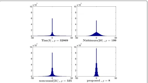
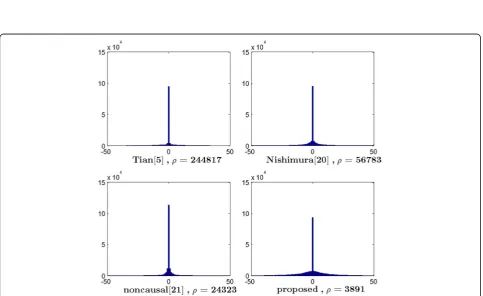
Figures 10, 11, 12, and 13 plot the histograms of the proposed predictor, DE predictor [5], linear predictor [20], and noncausal predictor [21] by using the four clips marked by 39, 49, 64, and 66, respectively. We can see that the proposed predictor provides the smallest error power and the prediction errors are closer to zero. The error power of the other schemes can be estimated by (17), whereNis the length of the audio file. For the other clips, the simulation results are similar. That means the pro-posed predictor can better reduce prediction errors. The main reason is that the proposed prediction model can better explore the correlation property of the samples for different types of audio files.
ρ¼ 1
N XN
i¼1
e2i ð17Þ
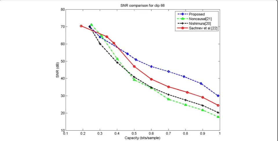
For the four example clips, we test the performance of the proposed scheme against three existing state of
the art works [20–22]. The method [22] proposed for
two-dimensional image files can be adapted for one-dimensional audio clips by rounding the average of two neighboring samples as the predicted value. Figures 14, 15, 16, and 17 plot the experimental results on four clips. We can see that for the same embedding capacity, the proposed scheme obtains the highest SNR values than the other three schemes. The basic reason is that we can use different orders of predictors to reduce the prediction error in noncausal way for different types of clips. In the previous schemes, the order of the pre-dictor is fixed for different clips or only past samples are used as prediction context. Similarly, from Figs. 18, 19, 20, and 21, our method has the highest ODG values than the other three schemes on the four example clips. Figure 22 shows the SNR results on 70 audio clips by 1 bit per sample. We can see that in most audio files, our method has the highest SNR. That means our pre-diction model has the least distortion for most of the clips. Figure 23 shows the ODG experimental results on 70 audio clips by 1 bit per sample. As we can see, lower ODG can be achieved for most of the clips.
Table 2 shows the average ODG value, average SNR value, the percentage of the best SNR values and the percentage of the best ODG values in all the 70 audio clips. We can see that the proposed method has the best performances for most of the clips.
Table 2SNR and ODG comparison for 70 audio clips
Schemes Average SNR Average ODG
Percentage of the best SNR
Percentage of the best ODG
Proposed 40.7 −1.24 90 76
Sachnev [22] 33.0 −1.53 7 1
Nishimura [20] 33.9 −1.58 3 16
Noncausal [21] 31.7 −1.61 0 7
Table 3Computational cost and decoding cost of the proposed scheme in the embedding
Clips Clip39 Clip49 Clip64 Clip66
Duration 2:17 0:22 0:30 0.17
Comp. cost by proposed 49:05 5:20 15:48 4:12
Comp. cost by [20] 0:12 0:06 0:06 0:06
Comp. cost by [21] 0:05 0:01 0:01 0:01
Comp. cost by [22] 0:05 0:01 0:01 0:01
Dec. cost by proposed 0:06 0:01 0:01 0:01
Dec. cost by [20] 0:05 0:01 0:01 0:01
Dec. cost by [21] 0:05 0:01 0:01 0:01
By choosing four different types of clips, Table 3 lists their durations, computational costs in the embedding, and the computational cost in the extracting by using four reversible data hiding schemes. The test software is Matlab R2012a running with the computer of i5-4690K Processor and CPU Speed of 4.4 GHz. In the proposed scheme, the computational cost in the embedding phase is somewhat higher since the prediction orders and the prediction coefficients are needed to be estimated at first for data hiding. For clip 39 with duration of 2 min and 17 s, the embedding cost is 49 min and 5 s. And the computational cost is related to the duration. From the perspective of applications, higher computational cost in the embedding phase is acceptable since the authentica-tion process is implemented in the extracauthentica-tion phase. In the proposed scheme, the decoding process is satisfac-tory since the auxiliary information has been restored for blind extraction.
4 Conclusions
The paper presents a reversible audio data hiding scheme by using noncausal prediction with alterable order. For an audio clip, the optimum order and the prediction coeffi-cients can be achieved by using the minimum error power method. As a result, the proposed prediction model can better explore the correlation of the samples. Experimen-tal results have shown that the proposed prediction model provides a satisfactory prediction precision for different types of clips. And, the proposed scheme (by combining the double-embedding strategy and the proposed predic-tion model) has lower embedding distorpredic-tion for the same embedding rate in comparison with several existing excel-lent works.
Funding
This work was partially supported by the NSFC project (No. 61272414), co-funded by the State Key Laboratory of Information Security (No. 2016-MS-07).
Competing interests
The authors declare that they have no competing interests.
Received: 6 August 2016 Accepted: 8 February 2017
References
1. YQ Shi, Z Ni, D Zou, C Liang, G Xuan, Lossless data hiding: fundamentals, algorithms and applications, inProc. IEEE ISCAS, vol. 2, 2004, pp. 313–336 2. J Fridrich, M Goljan, R Du, Invertible authentication, inProc. SPIE Security
Watermarking Multimedia Contents, San Jose, CA, 2001, pp. 197–208 3. J Fridrich, M Goljan, R Du, Lossless data embedding-new paradigm in digital
watermarking. Eurosip. J. Appl. Signal Process.2002(2), 185–196 (2002) 4. MU Celik, G Sharma, AM Teklap, E Saber, Lossless generalized-LSB data embedding, inIEEE Transactions on Image Processing, vol. 14, 2nd edn., 2005, pp. 253–266
5. J Tian, Reversible data embedding using a difference expansion, inEEE Transactions on Circuits and Systems for Video Technology, vol. 13, 8th edn., 2003, pp. 890–896
6. AM Alattar, Reversible watermark using difference expansion of triplets, in
Proc. Int. Conf. Image Process., vol. 1. Barcelona, Spain, 2003, pp. 501–504
7. HJ Kim, V Sachnev, YQ Shi, J Nam, HG Choo, A novel difference expansion transform for reversible data embedding, inIEEE Transactions on Information Forensics and Security, vol. 4, 3rd edn., 2008, p. 465
8. X Wang, X Li, B Yang, Z Guo, Efficient generalized integer transform for reversible watermarking, inIEEE Signal Processing Letters. 6, vol. 17, 2010, pp. 567–570
9. F Peng, X Li, B Yang, Adaptive reversible data hiding scheme based on integer transform. Signal Process.92(1), 54–62 (2012)
10. DM Thodi, JJ Rodriguez, Reversible watermarking by prediction-error expansion, inProc. IEEE Southwest Symp. Image Anal. Interpretation, Lake Tahoe, CA, 2004, pp. 21–25
11. DM Thodi, JJ Rodriguez, Expansion embedding techniques for reversible watermarking, inIEEE Transactions on Image Processing, vol. 16, 3rd edn., 2007, pp. 721–730
12. B Ou, X Li, Y Zhao, R Ni, Reversible data hiding scheme based on pde predictor. J. Syst. Softw.86(10), 54–62 (2012)
13. Y Hu, HK Lee, J Li, DE-based reversible data hiding with improved overflow location map, inIEEE Transactions on Circuits and Systems for Video Technology, vol. 19, 2nd edn., 2009, pp. 250–260
14. C Panyindee, C Pintavirooj, Optimizations using the genetic algorithm for reversible watermarking, inProc. ECTI-CON, 2013, pp. 1–5
15. S Kang, HJ Hwang, HJ Kim, Reversible watermark using an accurate predictor and sorter based on payload balancing, inETRI, vol. 34, 3rd edn., 2012, pp. 410–420
16. Z Ni, YQ Shi, N Ansari, S Wei, Reversible data hiding, inIEEE Transactions on Circuits and Systems for Video Technology, vol. 16, 3rd edn., 2006, pp. 354–362 17. M. Kamran, A. Khan, and S. A. Malik, A high capacity reversible watermarking
approach for authenticating images: exploiting downsampling, histogram processing, and block selection. Inf. Sci. (2013). doi: 10.1016/j.ins.2013.07.035 18. WL Tai, CM Yeh, CC Chang, Reversible data hiding based on histogram
modification of pixel differences, inIEEE Transactions on Circuits and Systems for Video Technology, vol. 19, 6th edn., 2009, pp. 906–910
19. D Yan, R Wang, Reversible data hiding for audio based on prediction error expansion, inProc. of IIHMSP2008, 2008, pp. 249–252
20. A Nishimura, Reversible audio data hiding using linear prediction and error expansion, inProc. of IIHMSP2011, 2011, pp. 318–321
21. S Xiang, Non-integer expansion embedding for prediction-based reversible watermarking, inProc. 14th Int. Conf, 2012, pp. 224–239
22. V Sachnev, HJ Kim, J Nam, S Suresh, YQ Shi, Reversible data embedding using sorting and prediction, inIEEE Transactions on Circuits and Systems for Video Technology, vol. 19, 7th edn., 2009, pp. 989–999
23. X Hu, W Zhang, X Li, N Yu, Minimum rate prediction and optimized histograms modification for reversible data hiding, inIEEE Transactions on Information Forensics and Security, vol. 10, 3rd edn., 2015, pp. 653–664 24. AH Nuttal, Spectral analysis of a univariate process with bad data points, via
maximum entropy and linear predictive techniques, inTech. Pep. TR - 5303, Naval Underwater Systems Center, New London, Conn, 1976
25. EBU Committee: sound quality assessment material recordings for subjective tests [online]. Available: https://tech.ebu.ch/publications/sqamcd
Submit your manuscript to a
journal and benefi t from:
7Convenient online submission 7Rigorous peer review
7Immediate publication on acceptance 7Open access: articles freely available online 7High visibility within the fi eld
7Retaining the copyright to your article
Submit your next manuscript at 7 springeropen.com