Application of the Modified Inverse Design Method in the Optimization of the Runner Blade of a Mixed-Flow Pump

ORIGINAL ARTICLE

Application of the Modified Inverse

Design Method in the Optimization

of the Runner Blade of a Mixed-Flow Pump

Ye‑Ming Lu

_{, Xiao‑Fang Wang}

_{, Wei Wang}

_{and Fang‑Ming Zhou}

Abstract

To improve the design speed and reduce the design cost for the previous blade design method, a modified inverse design method is presented. In the new method, after a series of physical and mathematical simplifications, a sail‑like constrained area is proposed, which can be used to configure different runner blade shapes. Then, the new method is applied to redesign and optimize the runner blade of the scale core component of the 1400‑MW canned nuclear coolant pump in an established multi‑optimization system compromising the Computational Fluid Dynamics (CFD) analysis, the Response Surface Methodology (RSM) and the Non‑dominated Sorting Genetic Algorithm‑II (NSGA‑II). After the execution of the optimization procedure, three optimal samples were ultimately obtained. Then, through comparative analysis using the target runner blade, it was found that the maximum efficiency improvement reached 1.6%, while the head improvement was about 10%. Overall, a promising runner blade inverse design method which will benefit the hydraulic design of the mixed‑flow pump has been proposed.

Keywords: Optimization, Mixed‑flow pump, Inverse design method, Runner blade, Nuclear coolant

© The Author(s) 2018. This article is distributed under the terms of the Creative Commons Attribution 4.0 International License (http://creat iveco mmons .org/licen ses/by/4.0/), which permits unrestricted use, distribution, and reproduction in any medium, provided you give appropriate credit to the original author(s) and the source, provide a link to the Creative Commons license, and indicate if changes were made.

1 Introduction

Mixed-flow pumps have the characteristics of both cen-trifugal pumps and axial pumps. They are widely used in various areas, such as industrial chemistry, industrial water applications, nuclear industry. As the heart of the power equipment in these areas, mixed-flow pumps can provide stable energy for the circulation of fluid medium. The need for designing a higher efficiency pump with lower energy consumption is increasing with the current advocacy for green power, nowadays [1]. Accordingly, an effective design method for configuring the runner blade of the pump for high efficiency and reasonable high head would be valuable.

To design and optimize the blade shape, the distribu-tion of the structural parameters, for instance the blade angles, were directly adjusted in previous studies [2–4]. Unfortunately, this approach is highly dependent on the

designers’ experiences. Additionally, a fair number of design parameters would need to be selected to be opti-mized in order to get a new runner blade that is quite different from the target. Instead of geometrically opti-mizing the blade with blade angles, an important inverse design method was proposed by Borges [5] to design a blade under incompressible conditions, which was sub-sequently extended to compressible conditions by Zan-geneh [6, 7]. In this inverse design approach, the blade shape was represented as sheets of blade loading with the approximate distribution controlled by specific vari-ables at the hub and shroud sides, such a design method has already been adopted in the TURBODesign software. Using this sequential design method in the software, several optimal pumps have been successfully obtained [8, 9]. However, some problems still remain waiting to be solved. First, the blade shape is simply controlled by two cross sections, namely, the hub section and the shroud section, and this so-called 2D blade profile can only configure a blade with straight leading edge instead of a complex bend leading edge. Nevertheless, the lead-ing edge affects the cavitation and secondary flows [10],

Open Access

*Correspondence: [email protected]

1 _{School of Energy and Power Engineering, Dalian University}

of Technology, Dalian 116000, China

thus a design method which can present a complex lead-ing edge would offer extra choices for improvlead-ing the flow characteristics. Moreover, the ranges for the design vari-ables are not clearly defined. Taking the design method in the TURBODesign software as an example, seven inde-pendent variables [8, 9], namely, NCs, NCh, NDs, NDh, SLOPEh, SLOPEs, LEh and LEs, are adopted, and with-out obvious definition for the range of these variables, a large number of samples would have to be generated before optimization, which would require a considerable amount of time and computing resource.

The shortcomings of the previous design methods, thus indicates that the more cross sections controlling the blade shape (for configuring the complex blade) and the fewer design variables (for quickly designing blade), the better the design method would be. However, the number of cross sections and the number of variables have an inverse proportional relationship. In some tradi-tional design methods [11], even four or five cross sec-tions are adopted, but they can just configure a few blade shapes due to the excessive number of variables located on the cross sections. To increase the control sections and decrease the number of variables, a modified design method based on the previous research is proposed here. The scholars associated with such research proposed the idea of using swirl velocity distribution to design the run-ner blade and have carried out relevant works [12, 13]. However, hardly any optimization work has adopted this method before. Besides, Bing [14] tried to specify the constrained variables to control the swirl velocity distri-bution, but the design variables have not been effectively limited. As for the modified design method in this paper, a sail-like constrained area controlling the design vari-ables is deduced by some physical and mathematical sim-plifications based on Bing’s work, using just three points located in the constrained area are used to configure the blade by controlling the cross sections. Ultimately, the modified inverse design method is effectively applied in a multi-optimization system to verify its effectiveness.

2 Modified Inverse Design Method

The Quasi-three-dimensional (Q3D) method which takes limited time and has successfully been applied to design the blade in previous studies [9, 12]. As for the Q3D the-ory, instead of taking the iteration computation of the S1 surface (blade-to-blade) and S2 (hub-to-shroud) surface, it takes the representative mean S2 surface (S2m) to pro-vide variables for the calculation of the S1 surface in the iterative process. To get the flow variables on the S2m sur-face, the preliminary calculation was performed by the given meridional shape, the blocking factor (determined by the blade numbers, blade thickness, etc.), operating conditions (including mass flow, temperature, pressure,

etc.) according to the 2-D streamline curvature method [15, 16] or Computational Fluid Dynamics (CFD) [17]. Compared with the 2-D streamline curvature method, the CFD method is much more accurate [17], thus, it was adopted here to calculate the average-wised variables on S2m surface.

2.1 Basic Runner Blade Design Theory

To design the impeller of a mixed-flow pump, the follow-ing factors need to be considered: (I) meridional channel shape including a leading contour; (II) blade thickness; (III) blade number; (IV) staking condition; (V) load-ing pressure [9] or swirl velocity [12, 17]. As mentioned in the title, this study is mainly concerned with design-ing the blade, so that factor (I) and factor (III) remain the same as the original target impeller which will be intro-duced in Section 4.1. When compared with other fac-tors, factor (II) has a faintness influence, so it was kept unchanged. As for factor (IV), the blade shape here can be controlled by three cross sections consisting of the hub side, the middle and the shroud side, which is shown in Figure 1(b). In Zangeneh’s design theory, the loading pressure of factor (V) is given as follows [6, 7]:

where p+ and p− represent static pressure on the pres-sure and suction side of the blade, B is the blade number,

ρ is the density and Vm is the pitch-wise averaged

meridi-onal velocity on the S2m surface.

Regarding Zangenh’s theory, after settling down the meridian shape, blade thickness and blade number, the preliminary averaged meridional velocity can be calcu-lated at first. And with the preliminary meridional veloc-ity and a given distribution of swirl velocveloc-ity, the loading pressure can then be calculated to configure the blade shape according to Eq.  (1). Afterwards, with the newly configured blade, the meridional velocity can be recalcu-lated. Additionally, the configured blade can be subjected to minor modifications according to the new meridional velocity and the established swirl velocity before. With the iterative modification above, the blade shape can be finally established until the variables remain stable.

As a result, the averaged meridional velocity is the intermediate variable and becomes gradually stable dur-ing the design process above, so that the swirl velocity becomes the unique variable determining the loading pressure as well as the blade shape. Regarding the factor (V), the swirl velocity can also take the place of the load-ing pressure distribution in determinload-ing the runner blade shape [17].

(1) p+−p−=(2π/B)ρVm

Unlike Zangeneh’s design theory, which uses the loading pressure to design the blade shape, the new design method uses swirl velocity to directly deter-mine the geometric variables. Here, the distribution of the swirl velocity is established first, and then it is combined with another traditional equation instead of using Eq. (1). Such equation can calculate the wrap angles directly, and is given as [6, 12]:

where ω represents the rotation velocity of the pump, and r is the radial coordinate.

After the calculation of the wrap angles, the results are then imported into a three-dimensional modelling software among with the other established variables,

(2)

θ =

ωr2−rVθ(s) Vmr2

ds,

such as blade thickness, meridional shape and blade number. Accordingly, it can be concluded that the dis-tribution of swirl velocity is the key factor to design the runner blade shape, and its distribution law will be dis-cussed next.

2.2 Derivation of the Constrained Area

As mentioned above, swirl velocity plays an extremely important role in determining the blade shape on the con-dition that the meridional shape, blade thickness and blade number are settled first. The distribution for swirl velocity along streamline can be described as follows [14]:

where r1Vθ1 and r2Vθ2 denote the swirl velocity at the inlet and outlet respectively, g(s) is the non-dimensional swirl velocity. According to pre-design variables from the target and the one-dimensional theory, r1Vθ1 and r2Vθ2 can be determined by the following equations [18, 19]:

where β1 is the inlet blade angle and can be calculated by the established variables from the target pump; Hd is the design target head; Vm1 is the meridional velocity at the inlet; γ is the correction factor; ηh is the hydraulic effi-ciency; u1 is the circumferential velocity at the inlet.

Then, how to settle down the distribution of g(s) would be a crucial step for the calculation of the swirl velocity. Actually, g(s) can also be expressed by the quartic polyno-mial [17]:

where a,b,c,d,e represent the coefficients.

Figure 1(a) gives the physical distribution law for the dimensionless swirl velocity [17, 20], which ranges from 0 to 1 and has an increasing trend along streamline. The dis-tribution law can be expressed as the following mathemati-cal constraints:

(3)

rVθ(s)=r1Vθ1+g(s)(r2Vθ2−r1Vθ1),(0≤s≤1),

(4) r1Vθ1=r12ω−

Vm1r1

tanβ1 ,

(5)

r2Vθ2= (1+γ )gHd

ωηh

+r1Vθ1,

(6)

β1≈arctan V1m

u1 ,

(7) g(s)=as4+bs3+cs2+ds+e,

(8)

g(0)=0,

(9)

g(1)=1,

(10)

∂(g(0))/∂s=0(Kutta−Joukowski condition),

a Sketch presentation of the swirl velocity distribution

b Random selected streamline

25 50 75

Streamline location s/% 0 25 50 75 100 100

0

Random selected streamline

where Eq. (10) is from Ref. [6]; Eq. (11) is from Ref. [17]; Eq. (12) is from Ref. [14].

With the combination of Eqs.  (7)‒(13), they can be further simplified as:

From Eq. (14), it is established that the other coeffi-cients b,c,d,e can be established by a given P, a, so that the distribution of g(s) is solved when the values of P, a are determined. Moreover, according to the range of s, inequalities in Eq. (14) can be further simplified as:

where max f1(s)

, min f1(s)

and min f2(s)

in Eq.  (15) are controlled by P, which is shown in Figure 2. The data in Figure 2(b) reveal that: as P ranges from 0 to 2.882, there is only one area marked in Figure 2(b) satisfying the constraint inequalities in Eq. (15), while, no other areas can meet the constraints with the change of P.

Overall, to satisfy the physical distribution law, the distribution of the swirl velocity along the streamline is eventually deduced as:

where r1Vθ1 and r2Vθ2 are calculated by the established variables from the target, and (P,a) can be selected from the sail-like constrained area in Figure 2(b) to determine the swirl velocity distribution.

2.3 Application of the Constrained Area in the Design Theory

Based on the previous discussion, three cross sections were applied here to configure the runner blade of the

(11) ∂(g(1))/∂s=P, (Pis constant, P≥0),

(12) ∂(g(s))/∂s|s∈[0,1]≥0,

(13)

g(s)|_s∈[0,1]≤1.

(14)             

b= −2a+P−2,c=a−P+3, d=0,e=0,

(s−1)(2s−1)a≥(3−1.5P)s+(P−3),

a≤ 1+(P−3)s

2_+(2−P)s3

s4_−2s3_+s2 ,

(15)                 

a≥max� f1(s)�

(0≤s<0.5),a≤min� f1(s)�

(0.5<s≤1),

a≤min� f2(s)�

(0<s<1),

f1(s)=(3−1.5P)s+(P−3) (s−1)(2s−1) ,

f2(s)=1+(P−3)s

2_+(2−P)s3

s4_−2s3_+s2 ,

(16)

rVθ(s)=r1Vθ1+g(s)(r2Vθ2−r1Vθ1) (0≤s≤1),

g(s)=as5+(−2a+P−2)s4+(a−P+3)s3,

mixed-flow pump, which is shown in Figure 3(a). The results indicate that each cross section is controlled by ten wrap angles. According to Eq. (2), the wrap angle of the jth point for these cross sections can be calculated as:

(17)                           

θh,j= j �

i=1

ωr_h,i2 −(rVθ(s))_h,i

V_m,h,ir_h,i2 ,

θm,j= j �

i=1

ωr_m,i2 −(rVθ(s))_m,i

Vm,m,ir_h,i2

,

θs,j= j �

i=1

ωr_s,i2 −(rVθ(s))_s,i

Vm,s,ir2_s,i ,

where θ_h,j , θm,j and θs,j are the wrap angles at the hub,

middle and shroud side respectively.

The design variables to control the blade shape are given in Figure 3(b). The variables are selected from the sail-like constrained area, and they are then used to establish the swirl velocity with Eq. (16).

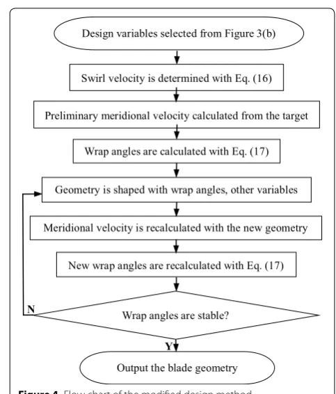
As previously mentioned, since the meridional shape, blade thickness, blade number, etc. from the target pump are settled, the preliminary averaged swirl velocity on the S2m can be calculated first. Based on the calculated meridional velocity, the established swirl velocity and other previously settled variables, the wrap angles can be obtained. After some iterate calculations above, the blade shape would finally be determined when the wrap angles become stable. The flow-chart for the design method is shown in Figure 4.

3 Multi‑optimization System

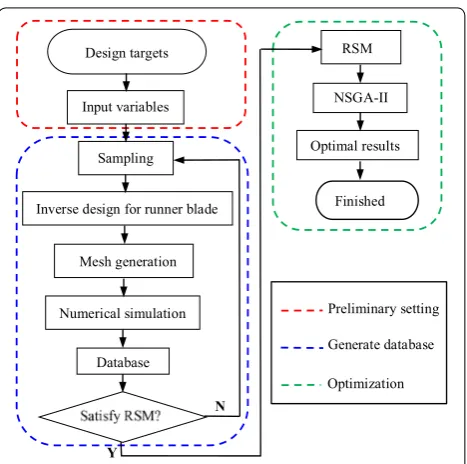
As shown in Figures 3(b) and 4, these design variables were randomly selected from the constrained area to generate the blade samples. Next, a multi-optimization strategy would be proposed to choose the right variables to optimize the runner blade. The previously reported design strategy [11, 24] is amended here to optimize the runner blade. The optimization strategy presented in Figure 5 consists of the modified inverse design method,

CFD analysis, RSM method and NSGA-II method. The details for the optimization process are as follows:

Step 1. Design targets that refer to the performances of the design impeller should catch up with the target pump at the set 0.8Q_d, 1.0Q_d and 1.2Q_d

mass flow conditions are set.

Step 2. The related design variables obtained from the target pump are input.

Step 3. A series of control design variables from the constrained area are selected to configure the blade shape by using the stratified sampling method and CFD analysis method.

Step 4. The mathematical relationships between the design variables and the objectives are estab-lished by using the RSM method.

Step 5. The right variables configuring the blade shape are chosen by applying the multi-objective algorithm NSGA-II.

3.1 Computational Fluid Dynamics (CFD) Analysis

3.1.1 Mesh Generation

After being configured by the inverse design method, the geometry was then imported into NUMECA/ Autogrid5. Taking into account the symmetry property a Wrap angles at the cross sections [19]

b Design variables from the sail-like constrained area Shroud

Middle

Hub

10.0

P

0 1 2 0 1 2 0 1 2

P

7.5

5.0

2.5

0.0

-2.5

B4 C4

A4

A3

A2

A1

B2

B1

C3

C2

C1

A(Ph,ah) C(Ps,as)

B3 B(Pm,am)

P

Figure 3 Wrap angles controlled by the design variables

Wrap angles are stable? N

Geometry is shaped with wrap angles, other variables Preliminary meridional velocity calculated from the target

Design variables selected from Figure 3(b)

Y

Output the blade geometry New wrap angles are recalculated with Eq. (17) Meridional velocity is recalculated with the new geometry

Wrap angles are calculated with Eq. (17) Swirl velocity is determined with Eq. (16)

of all blade passages in the pump, the flow character-istics of each blade passage can be considered to be the same. To reduce the grid number, it is necessary to select a single blade passage to simulate. The sin-gle blade passage is divided into several H blocks and I blocks with structured grids. To guarantee the qual-ity, the meshed grids must have the right orthogonality (> 15°), expansion factor (< 5) and aspect ratio (< 2000). Furthermore, to reach maximal y+ around 10 in the computational domains, the minimum height of the cells is controlled to be 0.005 mm at the walls.

3.1.2 Numerical Simulation

The meshed grids are then imported into NUMECA/ Fine. To simulate the three-dimensional viscous com-pressible turbulent flow in the passage, the continuity equation, energy conservation equation and Reynolds Navier–Stokes equation processed by the turbulent model are combined. On account of the properties with good stability, small calculation and high accu-racy, the Spalart–Allmaras turbulent model is chosen in the simulation process [21]. Moreover, with addi-tion of a second and forth order artificial dissipaaddi-tion, the second-order central scheme is adopted. The time marching is performed in a four-stage Runge–Kutta scheme, coupled with local time stepping and implicit residual smoothing technologies for convergence acceleration.

3.2 Optimization Process

3.2.1 Sampling Method

Due to its high response of non-linear fitting and good ability to fill space [22], the stratified sampling method is adopted here in the sampling process. By applying the stratified method, control design variables are ran-domly selected in the constrained area, so that it can systematically and integrally sample each subpopula-tion. With the combination of the stratified method and the inverse design method, the sampling procedure is described as follows:

Step 1. As shown in Section  2.3, the constrained

area at each cross section is divided into four equally small areas based on the equal area size. According to the data shown in this fig-ure, it can be identified from the bottom to the top as: the small areas at the hub side, which are denoted as A1,A2,A3,A4 one by one; the small areas at the middle, which are identified as B1,B2,B3,B4 ; and the areas at shroud side, which are designated as C1,C2,C3,C4.

Step 2. Continually, from the sail-like area, the

design variables A(P_h,a_h) , B(Pm,am) ,

C(Ps,as) are randomly sampled from the split areas Ai(i=1, 2, 3, 4) , Bj(j=1, 2, 3, 4) , and

Ck(k=1, 2, 3, 4) respectively. Based on the rule of permutation and combination, 43

sam-ples were obtained at the end, and the sample numbers are listed in the first row of the table found in the Appendix.

Step 3. After getting the sampled results of the design variables above, geometries for the runner blade were then configured with the inverse design method described in Section 2. Then, applying the CFD analysis method described in Section 3.1, the partial simulated perfor-mances of these samples were obtained and are also listed in the Appendix.

3.2.2 RSM Method

Regarding the engineering design process, it is almost impossible to exactly describe the functions between the input variables and output targets. Consequently, an approximate method must be used, and the RSM method is just the suitable one [8]. Accordingly, it is applied here to estimate the optimization targets. In order to make a relatively accurate description of the highly nonlinear relationships, the high order

Preliminary setting

Generate database

Optimization

Y

N

Design targets

Optimal results RSM

Finished NSGA-II

Satisfy RSM? Database Numerical simulation

Mesh generation Inverse design for runner blade

Sampling Input variables

polynomial model is adopted. The RSM model is given by the following equation [20]:

where ∧y _{is the output target,} ∂ denotes the coefficient, N is number of input variables and equals 6, the input varia-bles are: x1 is Ph , x2 is ah , x3 is Pm , x4 is am , x5 is Ps , x6 is as.

Generally, the prediction accuracy is highly depend-ent on the sample scale in the design space. As for the RSM model here, the least number of sample points is Smin=(N+1)(N+2)/2 . And N is 6 in this study,

therefore, Smin is 28. Since the number of samples in the database is 64 and exceeds 28, the sample scale satisfies the RSM prediction.

3.2.3 NSGA‑II Method

In view of the various conflicting optimization objec-tives, an effective multi-objective optimization algorithm is useful, and NSGA-II is just one of the ideal algorithms to perform this job. With the NSGA rooted in the arbi-trary sharing code, Det [9] came up with an effective modified algorithm NSGA-II, which combines the elitist-preserving approach and the crowding distance operator to maintain uniform and sustainable diversity. Previous studies relevant to the multi-optimization of the pumps have been carried out applying the NSGA-II method [9,

20]. The NSGA-II method is mainly divided into the fol-lowing steps.

Step 1. Initialize the random parent population of size

n, and predict the optimized targets with the RSM method.

Step 2. The parent individuals are classified by the non-dominated rank and crowding distance. Step 3. Individuals with higher crowding distance and

lower rank are preferred in the mating pool for generating the next generation.

Step 4. Simulated binary crossover and polynomial mutation are then applied with the crossover probability of 0.9 and mutation probability of 1/N (N is the number of variables, which is 6 here).

Step 5. After crossover and mutation, the mating pool generates a new generation of size n.

Step 6. Along with the preliminary population, the (18)

∧ y=∂0+

N

i=1 ∂1,ixi+

N

i=1 ∂2,ix2i +

N

i=1 ∂3,ix3i+

N

i=1

∂4,ix4i + N

i=1

∂5,ix5i + N

i=1 ∂6,ix6i,

whole population (size 2n) is reduced to size n

according to their rank and crowding distance. Step 7. Return to Step 2, and repeat the process until

the fixed generation is reached.

3.3 Optimization Targets

To guarantee the working range of the new runner blade, the pump efficiencies at 0.8Qd, 1.0Qd and 1.2Qd are set as the optimization targets:

where pt_out,pt_in are the total pressure at outlet and

inlet, respectively, Q is the volume flow, ω is the angular velocity, and τ is the torque.

Moreover, in order to improve the output energy, the head at the design point 1.0Qd should be considered at the same time. The head can be calculated as follows:

4 Optimization of the Runner Blade

4.1 Introduction to the Target Pump and Mesh Scheme

4.1.1 Target Pump

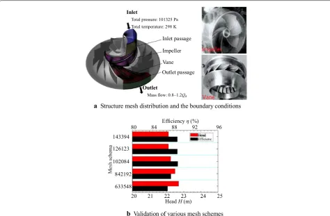
Regarding the target pump, it is taken from the core com-ponent of the scale hydraulic model 1400-MW canned nuclear coolant pump (on a scale of 1:2.5). The specific geometrical variables for the runner blade of the target mixed-flow pump are listed in Table 1. Also, the target pump has a rotation speed of 1495 r/min, and its design mass flow is Qd= 384 kg/s. The data shown in Figure 6(a) reveals that the target runner blade has a bend lead-ing edge. The boundary conditions of the target pump are shown in Figure 6(a). Moreover, previous research [23] has established that water can be used as the fluid medium in the evaluation of the performance of canned nuclear coolant pump. The hydraulic model here and the previously reported model [24] are from the same series with a relatively high performance, so that other details for the target pump can be obtained from the published paper.

4.1.2 Mesh Scheme and Its Validation

The target mixed-flow pump is set as the simulation model, and to exclude the effects of the grids and prove the stability of the simulation method, its validation will be performed first. Under the operating conditions stated above, five kinds of grids ranging from 633548 to 1433940 are chosen to be simulated under the design condition.

(19) ηi=

(pt_outi−pt_ini)×Qi τi×ω

(i=0.8, 1.0, 1.2),

(20) H1.0=

pt_out−pt_in

In addition, these grids satisfy the quality requirements described in Section 3.1, and the solver items are set as described in the same Part. The computational conver-gence is set below 10−6_{. The calculations were conducted} on a Dell Workstation with an Intel Core I5-6500 CPU.

The final simulation results of these grids are shown in Figure 6(b). According to the graph, when the num-ber of grids exceeds 1261236, the simulation result would remain stable. Thus, this kind of grid would be the appropriate grid scheme in the multi-optimization system. According to the numerical simulation results, the pump’s efficiency is ηd=90.4% , and its head is H_d = 22.1  m. Taking the simulating performance of the

target pump as the reference, the further optimization would be completed then.

4.2 Results for the Optimization Process

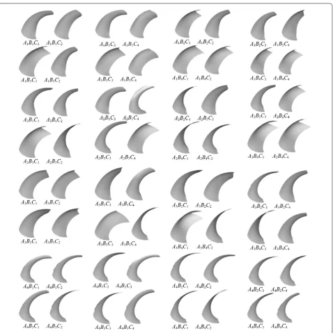
The results for each separate procedure, obtained through the application of the optimization process stated in Sec-tion 3, will be presented and discussed next. Using the sampling method in Section 3.2, Figure 7 shows the 64 generated samples in the database. Along with the perfor-mance of the samples, the wrap angle ranges at each cross section are also given in the table shown the Appendix. It can be inferred from these data that the modified design method could configure many blades with a wide range of blade shape, most importantly, these blades can also keep presenting good performances around the design point. Also, for these designed geometries with a relatively good performance, their wrap angles are increasing from the hub to the shroud gradually.

Additionally, through RSM analysis of the database presented in Figure 7, the mathematical relationships between the input design variables and the output per-formances were established. To show the reliability of RSM analysis, the R-square values are showed in Fig-ure 8. As for RSM, the closer to 1 the R-squared value is,

Table 1 Geometrical variables of the runner blade

Parameters Values

Inlet diameter D₁ (mm) 168

Outlet diameter D₂ (mm) 320

Wrap angle at hub θh (°) 0‒130

Wrap angle at middle θm (°) 0‒110

Wrap angle at shroud θs (°) 0‒92

a Structure mesh distribution and the boundary conditions

b Validation of various mesh schemes

Outlet passage Vane Impeller Inlet passage

Outlet

Mass flow: 0.8‒1.2Qd

Inlet

Total pressure: 101325 Pa Total temperature: 298 K

Head

80 84 88 92 96 Efficiencyη(%)

20 21 22 23 24 25 Head H(m)

Efficienc

143394 126123

842192 102084

633548

the higher the accuracy of the RSM model would be. The R-square values here are greater than 0.9, which indicates that the RSM has a faithful prediction accuracy. After obtaining the RSM functions, they are then applied in the optimization system along with the NSGA-II algorithm.

The basic setting of the NSGA-II algorithm is shown in Table 2. Apart from this basic setting listed in the NSGA-II, the design variables are A(Ph,ah) , B(Pm,am) and C(Ps,as) , which are selected from the sail-like

con-strained area of Section 2.3. Moreover, the efficiencies

at 0.8Qd, 1.0Qd, 1.2Qd ( η0.8 , η1.0 and η1.2 ) and head at design point ( H1.0 ) are selected to be the predicted per-formances of the generated samples in the optimization process. To enlarge the number of effective output sam-ples, the constraints for the predicted performances are also considered as follows: 0≤η0.8≤1 , 0≤η1.0≤1 ,

0≤η1.2≤1 , and Hd≤H1.0≤1.15Hd . The optimiza-tion objectives are the efficiency of the target pump at the three mass flow points, as shown in Table 3, their values are: ηt−0.8=79.7% , ηt−1.0=90.4% , ηt−1.2=88.1%.

A1B1C1 A1B1C2

A1B3C1 A1B3C2

A1B1C3 A1B1C4

A1B3C3 A1B3C4

A1B2C1 A1B2C2

A1B4C1 A1B4C2

A1B2C3 A1B2C4

A1B4C3 A1B4C4

A2B1C1 A2B1C2

A2B3C1 A2B3C2

A2B1C3 A2B1C4

A2B3C3 A2B3C4

A2B2C1 A2B2C2

A2B4C1 A2B4C2

A2B2C3 A2B2C4

A2B4C3 A2B4C4

A3B1C1 A3B1C2

A3B3C1 A3B3C2

A3B1C3 A3B1C4

A3B3C3 A3B3C4

A3B2C1 A3B2C2

A3B4C1 A3B4C2

A3B2C3 A3B2C4

A3B4C3 A3B4C4

A4B1C1 A4B1C2

A4B3C1 A4B3C2

A4B1C2 A4B1C3

A4B3C3 A4B3C4

A4B2C1 A4B2C2

A4B4C1 A4B4C2

A4B2C3 A4B2C4

A4B4C3 A4B4C4

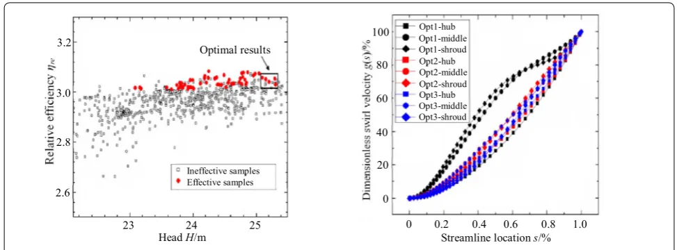
The NSGA-II process was finally executed using the settings above, and a total of 1000 different samples were ultimately obtained. To choose the optimal runner blades among these samples, a new combined variable was used to measure the efficiencies of 0.8Qd, 1.0Qd and 1.2Qd and is defined as follows:

Setting the defined η_re as the Y-axis, and the predicted design head H1.0 as the X-axis, the results shown in Fig-ure 9(a) were obtained and represent all samples obtained from NSGA-II. As for the samples, according to whether their predicted efficiencies exceed the efficiency of the target pump, they could be classified into effective sam-ples ( η0.8> ηt−0.8 and η1.0> ηt−1.0 and η1.2> ηt−1.2 ) and ineffective samples ( η0.8≤ηt−0.8 or η1.0≤ηt−1.0 or p+ ). From the results in Figure 9(a), it can be ascertained that about 8.0% of the samples’ efficiencies exceed those of the 1000 samples of the target impeller, and the optimal sam-ples would be among them.

Considering the predicted errors and to guarantee the improvement of the head on the off-design operating conditions near the design point, the optimal samples are to be chosen from the effective samples of a relatively

(21)

η_re= η0.8

ηt - 0.8

+ η1.0

ηt - 1.0

+ η1.2

ηt - 1.2 .

a Efficiency of 0.8Qdpoint b Efficiency of 1.0Qd c Efficiency of 1.2Qd d Efficiency of 1.2Qd

55 65 75 85

55 65 75 85

Actual η/%

R2_=0.989

Actual η/% 70 80 90

R2_=0.958

70 80 90

92

80 84 88 92 Actual η/%

R2_=0.902

80 84 86

28

24

16 20 24 28

Actual H/m

16 R

2_=0.976

20

Figure 8 Analysis of the R‑square error of RSM

Table 2 Basic setting of the NSGA‑II

Parameters Values

Number of generations 50

Population size 20

Crossover probability 0.9

Crossover distribution index 10

Mutation distribution index 20

Initialization mode Random

Max failed runs 5

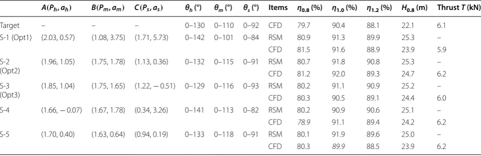
Table 3 Performances for the effective samples with relative high head

Italic values indicate the failure to meet the target performance

A(Ph,ah) Variables generating the hub angles; B(Pm,am) Variables generating the middle angles; C(Ps,as) Variables generating the shroud angles

A(Ph,ah) B(Pm,am) C(Ps,as) θh (°) θm (°) θs (°) Items η0.8 (%) η1.0 (%) η1.2 (%) H0.8 (m) Thrust T (kN)

Target – – – 0–130 0–110 0–92 CFD 79.7 90.4 88.1 22.1 6.1

S‑1 (Opt1) (2.03, 0.57) (1.08, 3.75) (1.71, 5.73) 0–142 0–101 0–84 RSM 80.9 91.3 89.9 25.3 –

CFD 81.5 91.6 88.9 23.9 5.9

S‑2

(Opt2) (1.96, 1.05) (1.75, 1.78) (1.13, 0.36) 0–132 0–115 0–91 _CFDRSM 80.7_{81.2 92.0}91.8 90.8_89.3 25.3_24.7 –_6.2 S‑3

(Opt3) (1.85, 1.04) (1.75, 1.65) (1.22, − 0.51) 0–129 0–116 0–93 _CFDRSM _80.380.2 91.1_90.5 90.9_89.1 25.2_24.4 –_6.0 S‑4 (1.66, − 0.07) (1.67, 1.78) (0.34, 3.26) 0–141 0–113 0–82 RSM 80.2 90.9 90.6 25.1 –

CFD 78.9 91.1 89.4 24.2 6.2

S‑5 (1.70, 0.40) (1.63, 0.64) (0.94, 0.19) 0–133 0–118 0–91 RSM 80.1 91.9 89.6 25.0 –

high predicted design head (25.0–25.5 m). The predicted performances for these effective samples with relative high heads were verified by CFD analysis, and the results are listed in Table 3. Regarding the five samples with relatively high head shown in Figure 9(a), Table 3 shows their performances predicted by the RSM and simulated by CFD. From the results in Table 3, it is established that the efficiencies of three samples at the monitor mass flow points exceed those of the target mixed-flow pump. Therefore, these three samples are chosen as the optimal samples, which are named as Opt1, Opt2 and Opt3. Most importantly, in Table 3, the axial thrust of the optimal results are very close to the target, which implies that they would not lead to any safety problems in the new design. The dimensionless swirl velocity distribution of the optimal samples is shown in Figure 9(b). Their char-acteristics will be further discussed along with the target pump.

4.3 Discussion of the Results

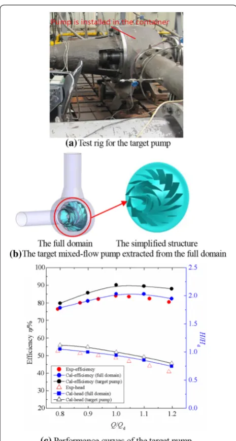
4.3.1 Experimental Validation for the Simulation

Sample performances in the optimization process above are mainly got by CFD analysis, though Section 4.1 has already excluded out the effect of grids, its accuracy should be further discussed. Taking the target impeller as the test model, the experimental verification was con-ducted on the test rig in Shenyang Blower Works.

The experimental results and those obtained by CFD analysis are shown in Figure 10. As shown in Figure 10(b), the target pump is extracted from the full domain of CAP1400. The simulation performances of the full domain as well as the simplified structure are presented in Figure 10(c). These results reveal that when compared

to the experimental results, the simulating results of the full domain are rather close to them, with results fall-ing within an error of 1% for the efficiency, and an error of 5% for the head at the design point. As the efficiency at the design point is rather close to the experimental result, the simulation results for the whole domain can be approximately used to evaluate the losses by compari-son of the simulation results of the simplified structure. Since the efficiency of the full domain is 85.2%, while the efficiency of the simplified structure is 90.2%, this clearly implies that about 5% loss occurred there. Nevertheless, it can be observed from the results in Figure 10 that the experimental and the simulation results have the same ascend and descend trends. Moreover, the experimental efficiency curve and the simulation efficiency curve have the same design mass flow point. Thus, the CFD analysis is reliable and it can be effectively applied in the optimi-zation process.

4.3.2 Comparison of the Characteristics

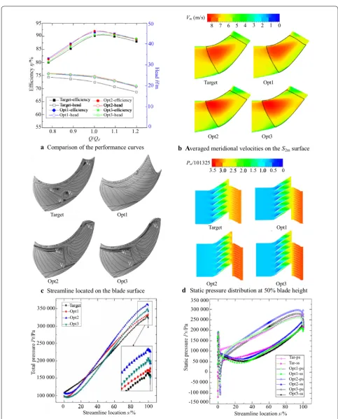
After the validation by CFD analysis, the simulation characteristics of the optimal samples and the target would be further discussed. The performance curves of the target pump and the optimal samples are pre-sented in Figure 11(a). According to the results shown in Figure 11(a) and Table 3, as the operating condition ranges from 0.8Qd to 1.2Qd mass flow, the efficiencies of the optimal samples are improved when compared with those of the target pump, especially the maxi-mum improvement in the design point, which can be as much as 1.6%. Additionally, at the design mass flow point, the heads of these optimal samples are increased a Classification of the predicted samples b The dimensionless swirl velocity of the optimal samples

2.6 2.8 3.0 3.2

23 24 25 Ineffective samples

Head H/m

Optimal results

Effective samples

0 0.2 0.4 0.6 0.8 1.0 Streamline location s/% 20

40 60

0 80 100

Opt3-shroud Opt1-middle Opt1-hub

Opt1-shroud Opt2-hub Opt2-middle Opt2-shroud Opt3-hub Opt3-middle

by 2.0 m, 2.6 m and 2.1 m, respectively, and the approx-imate head improvements can be as much as 10%. To verify the performance improvement, the inner flow analysis for the optimal and the target would be con-ducted next.

The averaged meridional velocities on the S2m sur-face are shown in Figure 11(b). These results indicate that that if the meridional shape, blade thickness, blade number, etc. from the target pump are settled, the aver-age meridional velocities of the newly designed blades continue exhibiting a similar distribution compared with the target. Accordingly, meridional velocity of the target could be employed for the newly design blades

as the initial before iterative design, which has already been discussed in Section 2.1.

The streamline distribution on the blade surface at the design point is shown in Figure 11(c). According to the results in this figure, there are four vortexes affecting the target pump’s blade surface, however, the vortexes disap-pear in terms of the Opt1 blade, and the number of vor-texes is decreased to three for the Opt2 and Opt3 blades. Most importantly, the vortex size is greatly decreased compared with the target. Since a vortex consists of a multitude of rotating flows, it really poses a threat to the stable inner flows and can also lead to unsteady forces on the runner blade [25, 26]. Therefore, as for the opti-mal samples, the reduction of the vortexes would lead to a performance improvement of the inner flows relative to the target pump.

To verify the head improvement in Figure 11(a), the results in Figure 11(d) show the static pressure distri-bution of the impeller and vane at 50% blade height. According to the results in this figure, the static pressure of the optimal samples increases orderly from the inlet of the impeller to the outlet of the vane. Furthermore, regarding the optimal samples, the outlet static pressure is higher than the target pump (the color is much redder), which indicates that the optimal samples have a higher work capacity.

Apart from the discussion for the static pressure, Fig-ure 11(e) shows the distribution of the quantitative total pressure along the streamline under the design condition. In this figure, at the outlet location, the total pressures of the optimal samples are larger than those of the target pump, which is consistent with the head improvement shown in Figure 11(a). Moreover, the pressure load of the optimal samples increased steadily along the streamline without any fluctuations, as shown in Figure 11(f), which means that the runner blades work on the flow medium continually without any distortions from the inlet to the outlet.

5 Conclusions

(1) For the modified inverse design method, a sail-like constrained area generating the design variables is derived after a series of mathematical simplifica-tions. Using a small scale of variables from the con-strained area, the blades are effectively configured. (2) Setting the scale core component of a 1400-MW

a Comparison of the performance curves

Target Opt1

Opt2 Opt3

c Streamline located on the blade surface

e Average total pressure distribution at 50% height

Target Opt1

Opt2 Opt3

b Averaged meridional velocities on the S2msurface

Target Opt1

Opt2 Opt3

d Static pressure distribution at 50% blade height

f Pressure load on the blade at 50% blade height

0 20 40 60 80 100

100 000 200 000

150 000

Streamline locations/%

250 000

300 000 Opt3

Opt2

350 000 Target_Opt1

55 60 65 70 75 80

0.8 0.9 1.0 1.1 1.2

Target-efficiency Target-head

Opt1-efficiency Opt2-headOpt3-efficiency Opt1-head Opt3-head

Opt2-efficiency

Q/Qd

85 95

90

300 000 350 000

-150 000 -100 000 -50 000 50 000 100 000 150 000 200 000 250 000

Streamline location s/%

Opt3-ss Opt3-psOpt2-ss Opt2-ps Opt1-ss Opt1-ps Tar-ssTar-ps

0

0 20 40 60 80 100

Pst/101325

3.0

3.5 2.5 2.0 1.5 1.0 0.5 0

3

Vm(m/s)

0

7 6 5 4 2 1

8

(3) The optimal samples are ultimately obtained after optimization. Through simulation and inner flow analysis, the performances are improved when compared to the target from 0.8Qd to 1.2Qd mass flow. At the design mass flow point, the maximum efficiency improvement is as much as 1.6%, and the design head is improved by about 10%.

Authors’ Contributions

F‑MZ and Y‑ML were in charge of the whole trial; Y‑ML wrote the manuscript; Y‑ML, X‑FW and WW assisted with sampling and laboratory analyses. All authors read and approved the final manuscript.

Author Details

1 _{School of Energy and Power Engineering, Dalian University of Technology,}

Dalian 116000, China. 2 _{Key Laboratory of Ocean Energy Utilization and Energy}

Conservation of Ministry of Education, Dalian University of Technology, Dalian 116000, China. 3 _{Collaborative Innovation Center of Major Machine}

Manufacturing in Liaoning Province, Dalian 116000, China.

Authors’ Information

Ye‑Ming Lu, born in 1991, is currently a PhD candidate at School of Energy and Power Engineering, Dalian University of Technology, China. He received his master degree from Tianjin University, China, in 2016, and his bachelor degree from Northwestern Polytechnical University, China, in 2013. His research interests include pump design and inner flow analysis of the unshroud centrifugal impeller

Xiao‑Fang Wang, born in 1961, is currently a professor at Dalian University of Technology, China. Her research interests include design and structural reli‑ ability analysis of turbomachinery.

Wei Wang, born in 1967, is currently an associate professor at Dalian Uni-versity of Technology, China. Her research interests include the cavitation study and inner flow analysis of fluid machinery.

Fang‑Ming Zhou, born in 1981, is currently a PhD candidate at School of Energy and Power Engineering, China. His research interests include the experi‑ mental investigation of the pump.

Competing Interests

The authors declare that they have no competing interests.

Funding

Supported by National Basic Research Program of China (973 Program, Grant No. 2015CB057301), Research and Innovation in Science and Technology Major Project of Liaoning Province, China (Grant No. 201410001), and Col‑ laborative Innovation Center of Major Machine Manufacturing in Liaoning Province, China.

Appendix Nomenclature

Symbols Names

p+ _{Static pressure on the pressure side} p− _{Static pressure on the suction side}

B Blade number

Vm Averaged meridional velocity

ω Pump rotation velocity

rVθ(s) Swirl velocity distribution along streamline

r1Vθ1 Swirl velocity at the blade inlet r2Vθ2 Swirl velocity at the blade outlet

g(s) Non‑dimensional swirl velocity

a,b,c,d Coefficients determining g(s)

β1 Blade angle at the inlet

A(Ph,ah) Design point generating the hub angles

θh,i Wrap angles at the hub

B(Pm,am) Design point generating the middle

angles

θm,i Wrap angles at the middle

C(Ps,as) Design point generating the shroud

angles

θs,i Wrap angles at the shroud

∧

y Output of the RSM

η Efficiency of the pump

H Head of the pump

p_in Total pressure at the inlet of the pump

p_out Total pressure at the outlet of the pump

τ Torque

Part B Generated samples in the database

No. A(P_h,a_h) B(Pm,am) C(Ps,as) η_0.8

(%) η(%)1.0 η(%)1.2 H1.0 (m) θh (°) θm (°) θs (°) Thrust (kN) T

A₁B₁C₁ (0.263, −1.273) (1.323, −1.016) (1.569, −0.838) 75.9 85.6 86.0 22.15 0−119 0−122 0−96 5.2

A₁B₁C₂ (0.629, −1.287) (0.493, −0.185) (0.196, 4.311) 75.1 87.4 86.7 23.20 0−130 0−112 0−79 5.8

A₁B₁C₃ (0.465, −0.727) (1.611, −0.774) (2.106, 2.341) 75.7 85.7 85.4 21.46 0−116 0−124 0−92 4.8

A₁B₁C₄ (0.917, −1.176) (0.141, −1.344) (1.558, 8.924) 77.0 89.1 86.6 22.82 0−136 0−113 0−77 4.7

A₁B₂C₁ (1.246, −0.313) (0.490, 2.855) (0.087, −1.395) 79.4 90.0 89.4 23.41 0−132 0−99 0−90 5.6

A₁B₂C₂ (0.094, −1.319) (0.726, 0.642) (0.275, 1.911) 74.8 88.6 88.7 24.70 0−115 0−110 0−84 5.7

A₁B₂C₃ (0.493, −0.185) (1.386, 2.241) (0.894, 4.510) 75.8 86.4 88.9 23.54 0~109 0−110 0−82 6.6

A₁B₂C₄ (0.913, 0.146) (0.413, 3.121) (1.027, 6.092) 71.9 90.0 90.4 24.95 0~116 0~97 0−80 6.3

A₁B₃C₁ (1.546, −0.158) (1.232, 3.745) (0.165, −2.123) 81.5 89.3 88.4 23.57 0−138 0−102 0−92 6.2

A₁B₃C₂ (0.087, −1.395) (1.451, 2.416) (0.110, 3.043) 76.8 88.9 88.9 24.81 0−116 0−109 0−81 6.3

A₁B₃C₃ (0.528, −2.284) (1.679, 3.709) (2.027, 3.862) 81.5 89.8 88.0 23.26 0−142 0−106 0−89 6.1

A₁B3C4 (1.246, −1.374) (2.131, 2.278) (1.833, 8.256) 80.0 88.8 85.6 21.19 0−149 0−117 0−83 5.0

A₁B₄C₁ (1.483, −0.565) (1.994, 5.056) (0.025, −0.823) 81.8 90.1 88,6 22.45 0−143 0−104 0−88 5.9

A₁B₄C₂ (0.412, −2.234) (2.110, 6.355) (1.255, 1.251) 81.1 89.0 88.8 21.78 0−138 0−100 0−90 5.1

A₁B₄C₃ (1.023, −0.032) (0.979, 6.199) (1.187, 4.725) 73.0 89.0 90.6 24.45 0−121 0−90 0−83 6.3

A₁B₄C₄ (1.513, −0.031) (1.256, 5.705) (0.755, 6.258) 75.3 90.0 89.2 24.13 0−136 0−95 0−78 5.9

A₂B₁C₁ (1.417, 1.897) (0.730, −0.249) (2.518, −0.186) 76.0 85.1 87.3 21.29 0−103 0−114 0−99 6.4

A₂B₁C₂ (1.142, 1.193) (0.219, 0.025) (0.611, 1.105) 69.9 84.7 88.0 23.14 0−106 0−108 0−87 5.5

A2B1C3 (0.346, 2.865) (1.313, 0.216) (2.164, 2.999) 65.4 77.3 85.7 19.16 0−60 0−117 0−91 5.5

A₂B₁C₄ (1.559, 1.036) (0.212, −0.148) (1.825, 5.965) 75.8 89.3 89.4 24.70 0−121 0−109 0−84 6.5

A₂B₂C₁ (0.722, 1.155) (0.020, 3.146) (0.257, −0.056) 67.7 79.2 89.0 21.34 0−95 0−93 0−88 5.2

A₂B₂C₂ (1.188, 2.233) (0.526, 1.420) (1.676, 1.026) 68.7 84.8 89.1 21.55 0−91 0−105 0−93 5.3

A₂B₂C₃ (1.386, 2.241) (0.502, 1.069) (2.373, 4.559) 69.5 84.3 89.2 21.95 0−97 0−107 0−89 6.5

A₂B₂C₄ (0.912, 0.812) (0.054, 2.925) (1.553, 6.846) 69.7 85.8 91.0 24.95 0−105 0−95 0−81 6.2

A₂B₃C₁ (2.005, 0.712) (1.280, 4.859) (0.278, 0.229) 80.3 89.3 90.2 23.66 0−139 0−98 0−87 6.3

A₂B₃C₂ (0.413, 0.824) (0.223, 4.813) (0.512, 2.613) 66.7 77.1 89.9 20.63 0−91 0−89 0−84 4.8

A₂B₃C₃ (0.571, 2.741) (1.642, 3.552) (1.851, 1.952) 66.3 79.4 88.4 19.54 0−66 0−107 0−92 5.2

A₂B₃C₄ (1.938, 0.449) (0.650, 4.111) (1.348, 5.543) 80.6 89.4 90.4 24.06 0−140 0−96 0−82 5.9

A₂B₄C₁ (0.657, 1.452) (1.523, 8.375) (0.039, 0.713) 67.3 77.5 88.2 20.48 0−88 0−86 0−86 7.7

A₂B₄C₂ (0.668, 1.919) (1.867, 6.503) (1.907, 1.789) 66.4 85.0 90.9 21.74 0−81 0−97 0−93 6.1

A₂B₄C₃ (1.959, 0.937) (1.404, 6.751) (2.164, 2.999) 75.4 89.7 90.6 23.35 0−133 0−92 0−91 5.4

A₂B4C4 (1.929, 0.766) (0.954, 5.832) (1.612, 6.011) 74.9 89.3 90.0 24.03 0−136 0−91 0−83 6.8

A₃B₁C₁ (2.319, 1.192) (0.501, −1.344) (0.976, −0.504) 80.1 90.6 89.7 26.71 0−140 0−116 0−93 6.8

A₃B₁C₂ (2.635, 1.962) (0.045, −0.048) (0.275, 1.911) 80.7 89.8 88.9 23.64 0−137 0−107 0−84 6.2

A₃B₁C₃ (2.031, 2.207) (0.015, 0.752) (1.025, 3.351) 71.9 86.6 89.5 24.69 0−116 0−103 0−85 5.8

A₃B₁C₄ (2.436, 3.973) (0.173, −0.400) (1.890, 8.957) 72.1 84.4 88.8 22.23 0−100 0−109 0−78 4.9

A₃B₂C₁ (2.083, 2.952) (0.512, 0.785) (1.012, −1.463) 71.1 85.4 89.0 22.93 0−106 0−108 0−96 5.7

A₃B₂C₂ (2.165, 1.407) (1.577, 1.351) (2.118, 1.007) 79.8 89.5 89.2 23.99 0−132 0−115 0−95 5.9

A3B2C3 (1.246, 4.246) (0.525, 3.079) (2.352, 2.546) 62.9 83.7 88.5 19.85 0−62 0−98 0−93 6.3

A₃B₂C₄ (1.921, 2.699) (1.316, 2.382) (1.809, 4.943) 74.2 85.7 88.6 22.87 0−105 0−108 0−86 5.8

A₃B₃C₁ (2.059, 1.498) (2.123, 1.958) (2.517, −0.200) 79.5 89.6 88.8 23.80 0−128 0−117 0−99 6.0

A₃B₃C₂ (2.089, 1.400) (1.920, 4.141) (1.884, 0.880) 80.1 89.5 89.6 23.89 0−130 0−107 0−94 6.1

A₃B₃C₃ (2.727, 0.904) (2.395, 3.463) (0.109, 4.294) 73.0 90.1 85.8 24.10 0−156 0−114 0−79 5.7

A₃B₃C₄ (1.091, 3.212) (0.354, 5.193) (1.553, 6.846) 63.1 78.4 89.8 19.76 0−73 0−88 0−80 5.6

A₃B₄C₁ (2.661, 1.896) (1.341, 6.847) (0.825, −1.371) 77.0 90.2 90.0 23.10 0−139 0−90 0−94 7.3

A₃B₄C₂ (1.862, 3.886) (1.244, 8.056) (0.500, 3.945) 65.8 76.4 90.2 20.04 0−85 0−84 0−81 5.6

No. A(Ph,ah) B(Pm,am) C(Ps,as) η0.8

(%) η(%)1.0 η(%)1.2 H1.0 (m) θh (°) θm (°) θs (°) Thrust (kN) T

A₃B₄C₄ (2.297, 3.414) (2.152, 4.868) (2.166, 4.488) 74.3 85.3 89.0 21.79 0−105 0−106 0−88 5.6

A₄B₁C₁ (1.921, 5.603) (1.120, 0.094) (1.246, −0.351) 64.8 80.5 85.4 19.58 0−60 0−116 0−93 5.5

A₄B₁C₂ (1.335, 5.055) (0.111, 0.194) (2.023, 0.424) 59.9 77.6 88.0 18.24 0−52 0−106 0−95 6.4

A₄B₁C₃ (2.265, 4.598) (0.110, −0.545) (2.715, 0.455) 69.7 83.9 88.5 21.13 0−86 0−109 0−99 6.5

A₄B₁C₄ (1.866, 5.587) (1.103, −0.923) (2.174, 5.232) 64.3 79.9 84.1 19.32 0−58 0−120 0−87 5.4

A₄B₂C₁ (2.125, 6.027) (0.116, 3.945) (2.185, 0.178) 61.6 76.8 87.3 16.62 0−59 0−91 0−97 7.2

A₄B₂C₂ (2.013, 4.835) (1.152, 2.063) (2.833, 0.023) 66.6 86.6 87.7 20.39 0−74 0−108 0−10 6.4

A₄B₂C₃ (2.223, 5.135) (0.201, 2.534) (2.574, 1.232) 64.9 83.1 89.6 19.36 0−76 0−98 0−97 6.7

A₄B2C4 (2.215, 4.735) (0.010, 2.843) (2.185, 5.322) 64.7 77.3 90.7 20.14 0−82 0−95 0−87 7.6

A₄B₃C₁ (1.875, 5.326) (1.521, 3.577) (1.902, 5.504) 64.4 78.8 87.8 18.50 0−63 0−105 0−85 8.1

A₄B₃C₂ (1.922, 5.935) (0.242, 4.858) (1.512, 1.755) 60.5 74.6 88.1 17.03 0−55 0−88 0−91 7.8

A₄B₃C₃ (1.350, 5.027) (0.192, 4.758) (2.212, 2.545) 60.4 73.3 88.3 16.47 0−52 0−87 0−92 7.6

A₄B₃C₄ (1.745, 5.526) (1.521, 3.577) (1.902, 5.504) 63.3 77.5 88.4 18.07 0−56 0−96 0−85 7.2

A₄B₄C₁ (1.621, 4.926) (1.205, 8.772) (0.025, 0.351) 61.6 71.9 80.5 16.27 0−62 0−81 0−88 7.9

A₄B₄C₂ (2.213, 4.946) (1.612, 9.526) (0.127, 3.092) 60.9 74.5 85.0 17.58 0−78 0−82 0−81 7.8

A4B4C3 (1.945, 5.758) (1.215, 6.578) (1.025, 3.845) 60.3 77.2 87.0 18.39 0−58 0−90 0−84 8.2

A₄B₄C₄ (1.221, 4.826) (1.524, 6.926) (1.313, 8.556) 59.8 75.4 86.5 18.02 0−51 0−92 0−76 7.0

Publisher’s Note

Springer Nature remains neutral with regard to jurisdictional claims in pub‑ lished maps and institutional affiliations.

Received: 16 March 2017 Accepted: 16 November 2018

References

[1] J H Kim, B M Cho, S Kim, et al. Design technique to improve the energy efficiency of a counter‑rotating type pump‑turbine. Renewable Energy, 2017, 101: 647–659.

[2] S Kim, K Y Lee, J H Kim, et al. High performance hydraulic design tech‑ niques of mixed‑flow pump impeller and diffuser. Journal of Mechanical Science & Technology, 2015, 29(1): 227–240.

[3] L H Liu, B S Zhu, L Bai, et al. Parametric design of an ultrahigh‑head pump‑turbine runner based on multiobjective optimization. Energies, 2017, 10(8): 1169.

[4] J S Anagnostopoulos. A fast numerical method for flow analysis and blade design in centrifugal pump impellers. Computers & Fluids, 2009, 38(2): 284–289.

[5] J E Borges. A three dimensional inverse method in turbomachin‑ ery: Part I—theory. ASME 1989 International Gas Turbine and Aero-engine Congress and Exposition, Toronto, Canada, June 4–8, 1989: V001T01A055–V001T01A055.

[6] M Zangeneh. A compressible three‑dimensional design method for radial and mixed flow turbomachinery blades. International Journal for Numerical Methods in Fluids, 2010, 13(5): 599–624.

[7] P Wang, M Zangeneh, B Richards, et al. Redesign of a compressor stage for a high‑performance electric supercharger in a heavily downsized engine. ASME Turbo Expo 2017: Turbomachinery Technical Conference and Exposition, Charlotte, USA, June 26–30, 2017: V008T26A027.

[8] B S Zhu, X Wang, L Tan, et al. Optimization design of a reversible pump‑ turbine runner with high efficiency and stability. Renewable Energy, 2015, 81: 366–376.

[9] R F Huang, X W Luo, J Bin, et al. Multi‑objective optimization of a mixed‑ flow pump impeller using modified NSGA‑II algorithm. Science China Technological Sciences, 2015, 58(12): 2122–2130.

[10] X J Li, Z Y Pan, D Q Zhang, et al. Centrifugal pump performance drop due to leading edge cavitation. IOP Conference Series: Earth and Environmental Science, London, UK, June 7–13, 2012: 032058.

[11] T Tuzson. Centrifugal pump design. 1st ed. New York: John Wiley & Sons, Inc., 1986.

[12] G Y Peng, S L Cao, M Ishizuka, et al. Design optimization of axial flow hydraulic turbine runner: Part I—an improved Q3D inverse method.

International Journal for Numerical Methods in Fluids, 2002, 39(6): 517–531. [13] G Y Peng, S L Cao, M Ishizuka, et al. Design optimization of axial flow

hydraulic turbine runner: Part II—multi‑objective constrained optimiza‑ tion method. International Journal for Numerical Methods in Fluids, 2002, 39(6): 533–548.

[14] H Bing, S L Cao, L Tan, et al. Parameterization of velocity moment distribu‑ tion and its effects on performance of mixed‑flow pump. Transactions of the Chinese Society of Agricultural Engineering, 2012, 28(13): 100–105. (in Chinese)

[15] V Pachidis, I Templalexis, P Pilidis. A dynamic convergence control algo‑ rithm for the solution of two‑dimensional streamline curvature methods.

ASME Turbo Expo 2009: Power for Land, Sea, and Air, Florida, USA, June 8–12, 2009: 287–296.

[16] M Casey, C Robinson. A new streamline curvature throughflow method for radial turbomachinery. Journal of Turbomachinery, 2010, 132(3): 031021.

[17] S L Cao, G Y Peng, Z Y Yu. Hydrodynamic design of rotodynamic pump impeller for multiphase pumping by combined approach of inverse design and CFD analysis. Journal of Fluids Engineering, 2005, 127(2): 330–338.

[18] N X Chen, Y L Wu. Centrifugal pumps. Beijing: China Machine Press, 2002. (in Chinese)

[19] Y M Lu, X F Wang, R Xie. Derivation of the mathematical approach to the radial pump’s meridional channel design based on the controlment of the medial axis. Mathematical Problems in Engineering. 2017, 2017(2): 1–16.

[20] J Pei, W J Wang, S Q Yuan. Multi‑point optimization on meridional shape of a centrifugal pump impeller for performance improvement. Journal of Mechanical Science and Technology, 2016, 30(11): 4949–4960.

[21] Y M Lu, Z X Liu. Quantitative analysis of influence factors on leakage flow of tip clearance in centrifugal impellers. Journal of Propulsion Technology, 2017, 38(1): 76–84. (in Chinese)

[22] G W Imbens, T Lancaster. Efficient estimation and stratified sampling.

Journal of Econometrics, 1996, 74(2): 289–318.

[24] H Gao, F Gao, X C Zhao, et al. Analysis of reactor coolant pump transient performance in primary coolant system during start‑up period. Annals of Nuclear Energy, 2013, 54(54): 202–208.

[25] S Kang. Numerical investigation of a high speed centrifugal compressor impeller. ASME Turbo Expo 2005: Power for Land, Sea, and Air, Nevada, USA, June 6–9, 2005: 813–821.