R E S E A R C H
Open Access
Room-localized speech activity detection
in multi-microphone smart homes
Panagiotis Giannoulis
1,3*, Gerasimos Potamianos
2,3and Petros Maragos
1,3Abstract
Voice-enabled interaction systems in domestic environments have attracted significant interest recently, being the focus of smart home research projects and commercial voice assistant home devices. Within the multi-module pipelines of such systems, speech activity detection (SAD) constitutes a crucial component, providing input to their activation and speech recognition subsystems. In typical multi-room domestic environments, SAD may also convey spatial intelligence to the interaction, in addition to its traditional temporal segmentation output, by assigning speech activity at the room level. Such room-localized SAD can, for example, disambiguate user command referents, allow localized system feedback, and enable parallel voice interaction sessions by multiple subjects in different rooms. In this paper, we investigate a room-localized SAD system for smart homes equipped with multiple microphones distributed in multiple rooms, significantly extending our earlier work. The system employs a two-stage algorithm, incorporating a set of hand-crafted features specially designed to discriminate room-inside vs. room-outside speech at its second stage, refining SAD hypotheses obtained at its first stage by traditional statistical modeling and acoustic front-end processing. Both algorithmic stages exploit multi-microphone information, combining it at the signal, feature, or decision level. The proposed approach is extensively evaluated on both simulated and real data recorded in a multi-room, multi-microphone smart home, significantly outperforming alternative baselines. Further, it remains robust to reduced microphone setups, while also comparing favorably to deep learning-based alternatives.
Keywords: Speech activity detection, Smart homes, Active room selection, Microphone arrays, Multi-channel fusion
1 Introduction
Smart home technology has been attracting increasing interest lately, mainly in assistive scenarios for the disabled or the elderly, but also in “edutainment”, home monitoring, and automation applications, among others [1–5]. Given that interaction with users must be convenient and nat-ural, and motivated by the fact that speech constitutes the primary means of human-to-human communication, voice-enabled interaction systems have been progressively entering the field. Indeed, multiple smart home projects have been focusing on voice-based interaction [6–13], and a number of commercial voice assistant home devices have recently been introduced in the market [14].
Such systems typically contain a sequence of modules in their architecture, with speech activity detection (SAD)
*Correspondence:[email protected]
1School of Electrical and Computer Engineering, National Technical University
of Athens, Athens, Greece
3Athena Research and Innovation Center, Marousi, Greece
Full list of author information is available at the end of the article
being a crucial one, as it provides input to other pipeline components, for example, speaker localization, speech enhancement, keyword spotting, and automatic speech recognition (ASR) [15–17], as well as contributing to the timing of the dialog management [18]. Further to voice-based interaction, SAD has found additional applications, such as telecommunications [19–21], variable rate speech coding [22], and voice-based speaker recognition [23,24], among others.
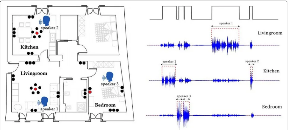
In practice, domestic environments contain multiple rooms, where one or more users may be located wishing to interact with the smart home voice interface. This sce-nario can be facilitated if the SAD module provides not only time boundaries of speech events (“when”), but also coarse speaker position (“where”) at the room level, i.e., assigning room “tags” to the detected speech activity, thus yielding separate speech/non-speech segmentation out-puts, one per room of the smart home (see also Fig.1). Enriching the traditional “room-independent SAD” to
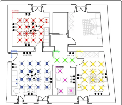
Fig. 1An example of room-independent vs. room-localized SAD in multi-room domestic environments equipped with multiple microphones. Here, three speakers are active in three rooms. Left: floor plan of the smart home used in the DIRHA project [10] (see also Section7.1and Fig.6), with dots indicating microphone locations on the apartment walls and ceiling. Right: 1-min-long waveforms, captured by the red-colored microphones (one per room with an active speaker), shown together with the corresponding ground truth of room-localized SAD. The room-independent
speech/non-speech segmentation is also depicted at the top
such “room-localized SAD” variant can be useful in mul-tiple ways: It can help disambiguate user commands for voice control of devices or appliances present in multiple rooms (e.g., light switches, windows, temperature control units, television sets); enable room-localized system feed-back, for example, via a loudspeaker or visual display at the room where speech activity takes place; and allow par-allel voice interaction sessions by multiple subjects inside different rooms, engaging separate system pipelines, one per room [16]; finally, ASR itself can benefit significantly from room localization [25].
Designing a robust SAD system in domestic environ-ments is a hard task due to the challenging acoustic con-ditions encountered. Such involve speech at low signal-to-noise ratio (SNR), presence of reverberation, and multiple background noise sources often overlapping with speech activity. In the case of room-localized SAD, these difficul-ties are further exacerbated due to acoustic interference between rooms. To counter these challenges, smart homes typically employ multiple microphones to capture the acoustic scene and “cover” the large multi-room interac-tion area. This allows exploiting multi-channel processing techniques, for example, fusion of the microphone infor-mation at the signal, feature, or decision level, in order to facilitate the analysis of the acoustic scene of interest.
Several efforts have been reported recently on room-localized SAD in multi-room environments [25–32] including our own work [33,34]. As further overviewed in Section2, these approaches vary in the kind of features,
classifiers, and number of microphones used per room. Depending on their design, they typically consist of one or two algorithmic stages, and may or not allow the detec-tion of simultaneously active speakers located in different rooms.
In this paper, we present our research work on room-localized SAD for smart homes equipped with mul-tiple microphones distributed in mulmul-tiple rooms. Our approach is based on the two-stage algorithmic frame-work that we originally proposed in [34]. There, room-independent SAD hypotheses, obtained at the first stage by traditional statistical modeling and acoustic front-end processing, are further refined and assigned to the room level at a second stage, by means of support vector machine (SVM) classifiers operating on a set of hand-crafted features that are suitably designed to discrim-inate room-inside vs. room-outside speech. The afore-mentioned approach is further extended in this paper in multiple ways. In particular:
• Concerning the first stage of the algorithm, this is modified to already provide room-localized SAD hypotheses, various choices for the set of its statisti-cal classes are investigated, and a number of multi-microphone decision fusion techniques are incorporated, which were originally studied in [35] for the problem of room-independent SAD only.
descriptor, as well as a source localization feature based on the smart home floor plan. Further, various feature fusion schemes across rooms are considered, accompa-nied by different options for their SVM-based modeling. Among these, one remains agnostic to the number of smart home rooms. In addition, application of the sec-ond algorithmic stage is also considered on medium-sized windows sliding over the first-stage hypothesized seg-ments, thus enabling their breakup and assignment to potentially different rooms.
•Finally, an extensive evaluation of all algorithmic com-ponents is reported, as well as of suitable alternative baselines including an extension of the seminal algorithm of [36] to the room-localized SAD problem. The experi-ments are conducted on a corpus of both real and sim-ulated data in a multi-room smart home, set up for the purposes of the DIRHA project [10]. This way, insights are gained concerning the strengths, weaknesses, and design choices of the proposed system. This is demon-strated to perform well in the challenging problem of room-localized SAD without the need of a large amount of training data, being robust to the number of available microphones, while also comparing favorably to alterna-tive deep learning approaches.
It should be noted that two of the aforementioned exten-sions have already been proposed in our earlier work [16], namely the room-localized operation at the first stage, as well as the sliding window mode at the second. However, since our focus there has been on the entire pipeline of the smart home spoken command recognition system, a contrastive evaluation of these enhancements for room-localized SAD has not been investigated. In particular, the room-localized operation at the first stage was also part of our system in [33], where however the focus lied on a joint SAD and speaker localization challenge over a limited area of a multi-room domestic environment [28].
The remainder of the paper is organized as follows: related work is summarized in Section 2; the overview of the proposed system is provided in Section 3, with its two algorithmic stages further detailed in Sections4 and 5; alternative baselines are presented in Section 6; the datasets and experimental framework are discussed in Section7; the evaluation is reported in Section8; and finally, conclusions are drawn in Section9.
2 Related work
SAD has been a topic of intense research activity, with numerous algorithms proposed in the literature over more than four decades, as for example overviewed in [37]. Some of the most established methods include algorithms incorporated into standards [20,21], the statistical model-based approach by Sohn et al. [36], and the spectral divergence proposed by Ramírez et al. [38], among oth-ers. Typically, SAD methods extract various features from
the waveform that are, for example, related to energy or zero-crossing rate [20,21,39,40], harmonicity and pitch [41–43], formant structure [20, 24, 44, 45], degree of stationarity of speech and noise [46–48], modulation [49–51], or Mel-frequency cepstral coefficients (MFCCs) [24]. Feature extraction is subsequently followed by tra-ditional statistical modeling or, more recently, by deep learning-based classifiers, for example, deep neural net-works (DNNs) [52, 53], recurrent ones [54,55], or volutional neural networks (CNNs) [56–58], often in con-junction with autoencoders [59]. Further, end-to-end deep learning approaches applied directly to the raw signal have also been proposed [60].
Specifically for the smart home domain, several SAD systems have been developed over the last decade, fol-lowing the collection of appropriate corpora in domestic environments [61–65]. For example, in [66], linear fre-quency cepstral coefficients are employed as features in conjunction with the Gaussian mixture model (GMM) and hidden Markov model (HMM) classifiers to detect distressed speech or acoustic events inside a smart apart-ment for elderly persons. In a similar task under the Sweet-Home project in [67], sound event detection is first performed by discrete wavelet transform features and an adaptive thresholding strategy, followed by speech/event classification using SVMs with GMM supervectors based on MFCCs. In [68], a simple energy-based SAD pre-cedes the HMM-based recognition of sounds and spoken words. In [69], SAD is performed on headset microphone audio to track human behavior inside a smart home, with the proposed system employing an energy detec-tor and a neural network trained on linear predictive coding coefficients and band-crossing features. Finally, in our earlier work within the DIRHA project [35], we investigated several fusion techniques for multi-channel SAD based on GMMs and HMMs trained on traditional MFCCs.
The aforementioned SAD systems aim to detect speech activity over the entire smart home, without however con-sidering its typical multi-room layout. Only few recent approaches in the literature focus on the task of room-localized SAD in multi-room domestic environments that constitutes the focus of this paper, yielding a speech/non-speech segmentation for each individual room of the smart home.
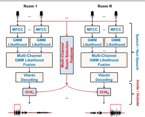
Fig. 2Block diagram of the proposed room-localized SAD system. The first-stage algorithmic components are depicted in blue and the second-stage ones in red
and concatenated to feed a linear discriminant analysis classifier that yields the segment room allocation. In [26], at the first stage, statistical-based SAD is performed for each microphone, and then, majority voting over the room microphones provides the speech segments of each room. At the second stage, speaker localization output feeds a classifier (SVM or neural network) to further examine speech segments and delete those originating in other rooms. In [27], at the first stage, multi-layer perceptrons are employed for each microphone, and speech/non-speech segmentation is achieved via majority voting for each room. Then, in case of segments assigned to multiple rooms, a speech envelope distortion measure is employed to decide the correct room. In [28], three different features are investigated for room-localized SAD, namely SNR, periodicity, and the global coherence field. Speech bound-aries for each room are computed by simple thresholding of these feature values and by using a heuristic rule over consecutive active frames.
In addition to the above, single-stage approaches have also been pursued for room-localized SAD. Specifi-cally, in [29], a DNN is employed taking as input 176-dimensional vectors composed of a variety of fea-tures, such as MFCCs, RASTA-PLPs, envelope variance, and pitch. Similar features (but 187-dimensional) and DNNs are again considered in [30], as well as alter-native classifiers, including a 2D-CNN. The latter is extended to a multi-channel 3D-CNN system in [31], where log-Mel filterbank energies (40-dimensional) are employed as features, temporal context is exploited by concatenating adjacent time frames, and the resulting 2D single-microphone feature matrices are stacked across
channels. Finally, in [32], the aforementioned 3D-CNN is combined with the GCC-PHAT [70] based CNN of [71] to yield a joint SAD and speaker localization network.
As already mentioned in the introduction, we have also investigated room-localized SAD in our earlier work, fol-lowing the two-stage algorithmic paradigm. Specifically, in [33], at the first stage of the developed approach, speech/non-speech segmentation was performed for each room, by means of multi-microphone decision fusion over GMMs trained on a traditional MFCC-based acoustic front-end. At the second stage, in case of speech seg-ments simultaneously active in multiple rooms, room selection was enabled by comparing an average GMM-based log-likelihood ratio for the given segment across the different rooms. In subsequent work [34], the first stage was replaced by a multi-channel room-independent SAD module, whereas the second stage adopted the use of specific features to discriminate inside vs. room-outside speech by means of SVM-based classifiers. The approach was further refined in later work [16], as part of a modular pipeline of a smart home spoken command recognition system.
In the current paper, we maintain the two-stage algo-rithmic approach for room-localized SAD, combining the design of the first stage in [33] with that of the second stage in [34]. In the process, we introduce a number of extensions in fusion techniques, hand-crafted room dis-criminant features, statistical modeling, and system eval-uation, as discussed earlier in Section 1. The resulting algorithm is presented in detail next.
3 Notation and system overview
Let us denote by R the number of rooms inside a given smart home that is equipped with a set of microphones Mall. This is partitioned into subsets Mr, for r = 1 , 2 ,. . .,R, each containing the microphones located inside room r. Let us also denote by om,t the short-time acoustic feature vectors (e.g., MFCCs) extracted from the signal of microphone m, and by oM,t their concatena-tion over microphone setM ⊆ Mall, with t indicating time indexing at the frame level (typically at a 10-ms resolution).
We are interested in room-localized SAD, seeking speech/non-speech segmentations for each room r, detecting speech events occurring inside it but ignor-ing speech originatignor-ing in other rooms or any other non-speech events. As also shown in Fig. 1, this differs from room-independent SAD, where a single speech/non-speech segmentation is produced, including speech/non-speech events occurring inside any of the R rooms of the smart home.
system for room-localized SAD operates in two stages. The first stage, detailed in Section4, is based on single-channel GMM classifiers, each trained on an individual room microphone, employing MFCC features and oper-ating at the frame level. An appropriate decision fusion scheme follows, combining GMM likelihood scores across all room microphones and, by means of Viterbi decod-ing, providing a crude speech/non-speech segmentation for the given room. Then, at the second stage, presented in detail in Section5, for the speech segments detected for each room, an SVM classifier is employed on a num-ber of hand-crafted room localization features, specially designed to discriminate room-inside vs. room-outside speech. Various feature fusion schemes across rooms are considered for this purpose, accompanied by different options for their SVM-based modeling.
4 First stage: speech segment generation
We now proceed with a detailed description of the first stage of the developed room-localized SAD system. This stage generates individual speech/non-speech segmen-tations for every room using the specific room micro-phones only, thus providing initial room-localized SAD hypotheses to be refined later. To accomplish this, it employs traditional acoustic front-end processing and sta-tistical modeling at the microphone level as discussed in Section4.1, followed by decision fusion across micro-phones as detailed in Section4.2and appropriate decod-ing schemes that are presented in Section4.3. Variations on the choices of microphones and classes considered are discussed in Section4.4.
4.1 Single-microphone system core
At the core of the system lies the single-microphone speech/non-speech modeling. Specifically, for each microphone of the smart home, a traditional 39-dimensional MFCC-plus-derivatives acoustic front-end is employed, with features extracted over 25-ms
Hamming-windowed signal frames with a 10-ms
shift. Subsequently, two-class microphone-specific GMMs are trained on these features (32 Gaussian mixtures with diagonal covariance matrices are used in our implementation), with the set of classes being J = {spr, silall}, where spr denotes speech originat-ing in room r where the given microphone is located and silall indicates the lack of speech in all rooms. Alternative class choices for set J are discussed in Section4.4.
4.2 Multi-microphone decision fusion
The developed system performs multi-microphone fusion at the decision level, where the GMM log-likelihood scores of different channels are combined at the
frame level for each class of interest, potentially also incorporating channel decision confidence. In particular, the following approaches for decision fusion over micro-phone setM⊆Mall are considered, which were investi-gated in our earlier work [35], but for room-independent SAD only:
• Log-likelihood summation, where the fused log-likelihoods (log class-conditionals) at frame t become
cM,j(oM,t) =
m∈M
wm,tbm,j(om,t), (1)
wherebm,j(om,t)denotes the log-likelihoods of the GMMs for microphonem given its acoustic featuresom,tat time frame t and class j ∈ J. The individual microphone scores in (1) can be uniformly weighted by setting wm,t= 1/|M| (where|•|denotes set cardinality), in which case the scheme will be referred to asunweighted log-likelihood
summation(“u-sum”), or adaptively weighted at any given
time framet, according to channel decision confidence that is estimated as
wm,t = |
bm, spr(om,t) − bm, silall(om,t)|
m∈M|
bm, spr(om,t) − bm, silall(om,t)|
, (2)
in which case, the method will be termed weighted
log-likelihood summation (“w-sum”). Weighting by (2) was
investigated among other schemes for room-independent SAD in [35], motivated by intuition that large log-likelihood differences between the classes imply higher classification confidence.
•Log-likelihood selection, where, at each time framet, a microphonemˆt ∈ M is selected to provide all fused class log-likelihoods, i.e.,
cM,j(oM,t) = bmˆt,j(omˆt,t), for all j∈J . (3) Such microphone can be chosen as the one achieving the highest frame log-likelihood over all channels and over all classes, i.e.,
ˆ
mt = arg max m∈M
max
j∈J bm,j(om,t)
,
in which case the scheme will be referred to as
log-likelihood maximum selection(“u-max”), or as the channel
with the highest confidence (2), i.e.,
ˆ
mt = arg max m∈M wm,t,
in which case the method will be termed log-likelihood
confidence selection(“w-max”).
case the scheme will be termedunweighted majority vot-ing (“u-vote”), or scaled by means of (2), resulting in
weighted majority voting(“w-vote”).
Among the above approaches, based on the experimen-tal results of Section 8, the developed room-localized SAD system employs the “w-sum” scheme computed over the set of microphones inside one room at a time, i.e., M = Mr. Alternative choices for set M are discussed in Section4.4.
4.3 Speech/non-speech segmentation
Following GMM training and multi-channel fusion, two speech detection implementations are developed: The first operates on mid-sized sliding windows, thus result-ing in low latency, whereas the second performs Viterbi decoding over longer sequences, providing superior accu-racy (as demonstrated in Section 8), but being more suitable for off-line processing.
• GMM-based scoring over sliding window: This scheme performs sequential classification over sliding windows of fixed duration and overlap (400 ms and 200 ms, respectively, are used). Specifically, for a given time windowT =[ts,te] and microphonem, the log-likelihoods for each class j ∈ J are first computed by adding all frame scores within the window. This results in scoresbm,j(om,T)=tte=tsbm,j(om,t), whereom,T denotes all feature vectors within windowT . Microphone fusion is then carried out as in Section4.2, but employing the window log-likelihoods instead.
•HMM-based Viterbi decoding over sequence: In this scheme, HMMs are built with a set of fully connected states J, state transition probabilities {ajj, for j,j ∈ J }, and class-conditional observation probabilities pro-vided by the class GMMs of Section 4.1. Then, Viterbi decoding is performed over an entire sequence of obser-vations (in our data, such are of 1-min length, as dis-cussed in Section 7.1), in order to provide the desired speech/non-speech segmentation. Specifically, for the single-microphone case, the well-known recursion [72]
δm,j(t) = max
j {δm,j(t−1) + log(ajj)} + bm,j(om,t), is used, where δm,j(t) denotes the score of the best decod-ing path enddecod-ing at state jand accounting for the first t
frame observations of microphonem. This can be read-ily extended to the fusion schemes of (1) and (3) over microphone setMas:
δM,j(t)=max j {δM,j
(t−1)+log(ajj)} +cM,j(oM,t), whereas majority voting fusion schemes “u-vote” and “w-vote” are modified to be applied over best-path scores
δm,j(t) instead of log-likelihoods bm,j(om,t).
Between the two aforementioned decoding schemes, the proposed system follows the HMM-based approach
due to its superior performance, with a number of fine-tuned parameters incorporated in it. Specifically, these are the state transition penalty that tunes the flexibility of the decoder to change states, as well as the speech class prior that favors or not the selection of the speech state.
4.4 Variations in sets of classes and microphones
As already discussed, to obtain the first stage of the speech/non-speech segmentation hypothesis for roomr, only the particular room microphones are considered (M = Mr). A number of variations however are possi-ble for the set of classesJ, which are investigated in the experiments of Section8.2:
• J = {spr, silall}, where spr denotes speech inside room r and silall indicates the absence of speech in all rooms of the smart home. This set is used in the proposed room-localized SAD algorithm.
• J = {spr, silr}, where silr indicates the absence of speech in roomr. This set is used in our work in [33].
• J={spr, spr¯, silall}, where sp¯r indicates the speech inside any of the other rooms, excluding room r.
In addition, in our earlier work [34], the first stage of the algorithm provides room-independent SAD out-put. That system uses the “w-sum” decision fusion scheme with all smart home microphones contribut-ing to (1), i.e., M = Mall. Further, the set of classes employed is J = {spall, silall}, where spall denotes the speech occurring in any of the smart home rooms.
5 Second stage: room assignment
Following the generation of initial room-localized SAD hypotheses, the second stage of the developed algorithm performs the final selection of active segments for each room. For this purpose, five hand-crafted features are pro-posed as detailed in Section5.1, extracted at the segment level for each room, and capable of segment discrim-ination as originating from inside vs. outside a given room. These features are then fused within and across rooms as presented in Section 5.2 and are fed to SVM classifiers that perform room assignment as detailed in Section5.3, temporally operating on the given segment as discussed in Section5.4. Various options for the above are presented.
5.1 Room discriminant features
As mentioned above, for any first-stage speech segment T =[ts,te] starting at time-frametsand ending at frame
with higher energy and lower reverberation than micro-phones located outside it. Likewise, the room door region typically appears as the speech source for room-outside segments.
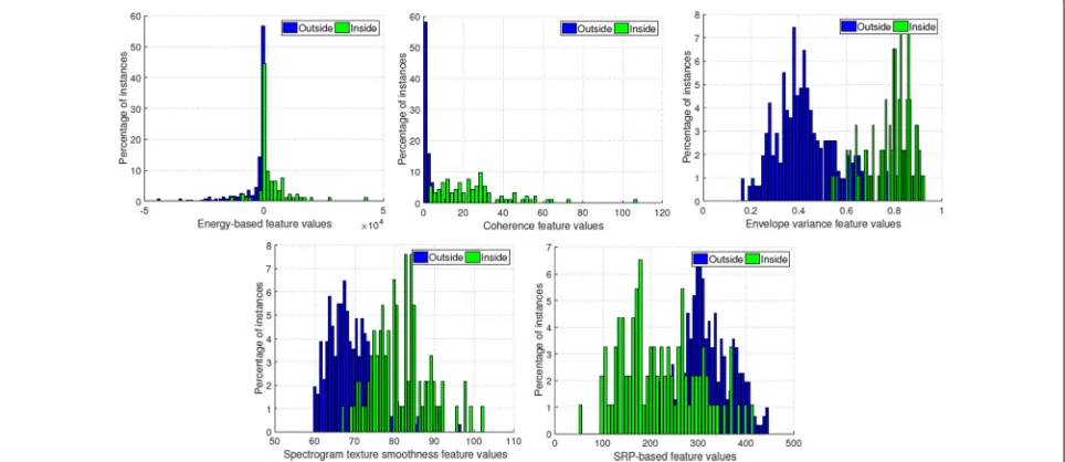
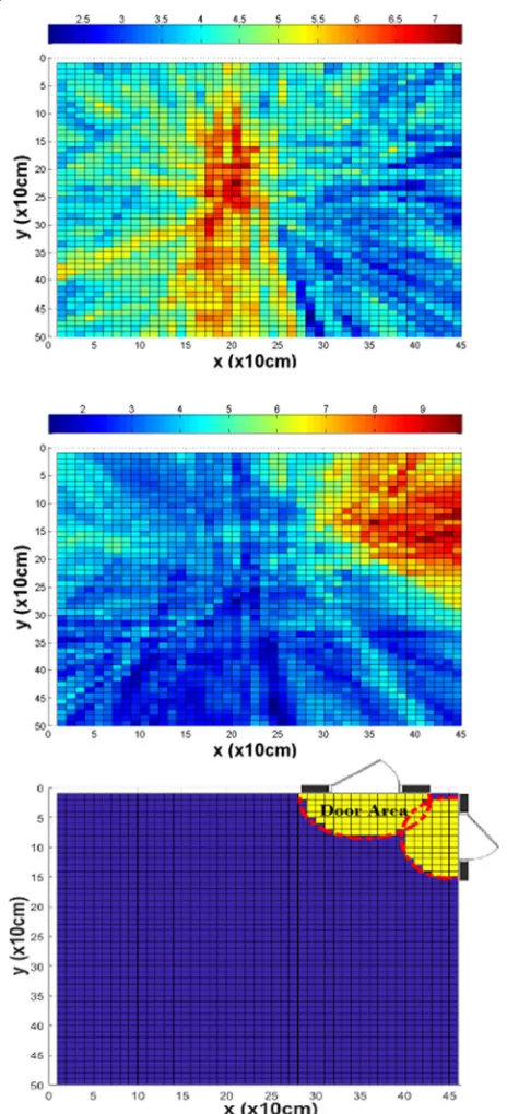
In particular, five scalar features are considered in this paper, extending our earlier work [33] with two addi-tional novel features presented in Sections5.1.4and5.1.5. The features are specially designed to provide room-inside vs. room-outside segment source discrimination, as also depicted in the histograms of Fig.3.
It should be noted that in contrast to the acoustic front-end of the first stage of the algorithm that extracts microphone-dependent features, the features of the sec-ond stage are instead room-dependent. Indeed, their esti-mation typically involves all microphones located in a room (or in the entire smart home, as in Sections5.1.1 and 5.1.3), performing in a sense fusion of their infor-mation at the signal level. Such derivation requires of course knowledge of the microphone room membership, but in the case of Section5.1.2also of additional informa-tion concerning which microphones lie adjacent to each other, and in the case of Section5.1.5further knowledge of the microphone topology and room layout. Details are provided next.
5.1.1 Energy-based feature
Originally proposed in [33], this feature is motivated by intuition that microphones inside the room where speech activity occurs will exhibit, on average, higher SNRs compared to ones outside it. For its computation, given detected speech segmentT =[ts,te] , the energy
ratio (ER) of speech over non-speech is first computed for all smart home microphones. For this purpose, the initial part of the speech segment, as well as the trailing part of non-speech preceding it, both of length τ, is utilized to yield
ERm,T =
⎛
⎝Lts+τ−1
τ=Lts
xm(τ)2
⎞ ⎠
⎛ ⎝Lts−1
τ=Lts−τ
xm(τ)2
⎞
⎠, (4)
for all microphones m ∈ Mall. In (4), xm(τ) denotes the signal captured by microphone m, with τ indicating indexing at the sample level. The latter is related to frame-level indexing by τ =L t, whereLis the number of signal samples over the short-time window shift. Following com-putations (4), the ERs are sorted across all smart home microphones, and the microphone set with theKlargest values is derived, denoted byM(K). Finally, the desired energy-based feature for room r is extracted as the differ-ence between the sum of the ERs of the microphones in setM(K)that are located inside roomrand the ER sum of the ones inM(K)but located in other rooms, namely
fr(,Ten) =
m∈M(K)∩Mr ERm,T −
m∈M(K)\Mr ERm,T ,
for all rooms r = 1 , 2 ,. . .,R. In our implementation,
K=5 and, in (4), τcorresponds to a 0.5-s interval. 5.1.2 Coherence feature
Originally proposed in [25] and re-used in [33], this fea-ture is motivated by intuition that signals capfea-tured by
Fig. 3Histograms of the five hand-crafted scalar features of Section5.1, demonstrating their ability to discriminate room-inside vs. room-outside speech. Histograms are computed over the development set of the simulated dataset of Section7.1, for the case of the smart home bedroom (see also Fig.1). Upper row, left-to-right: energy-based feature (Section5.1.1), coherence feature (Section5.1.2), and envelope variance one
pairs of adjacent microphones located outside a speech-active room will exhibit higher reverberation and thus lower cross-correlation than pairs inside it. To compute the coherence feature for room r, the set of adjacent pairs of microphones inside the room is first determined, denoted by {Mr × Mr}adj. Such pairs typically con-sist of neighboring microphones in larger arrays (see also Section7.1). Then, for every time frametwithin detected speech segment T , the maximum cross-correlation of the signal frames of adjacent microphone pair (m,m)
is computed, denoted by Cm,m(t). This is repeated for all pairs (m,m) ∈ {Mr × Mr}adj and the maximum retained. Finally, the result is averaged over the entire segment T , yielding the coherence feature for roomr, as:
fr(,Tcoh) = avg t∈T
⎧ ⎪ ⎨ ⎪ ⎩(mmax,m)
∈ {Mr×Mr}adj Cm,m(t)
⎫ ⎪ ⎬ ⎪ ⎭ .
Note that this feature employs the un-normalized cross-correlation function in order to also “capture” signal atten-uation. In our implementation, signal cross-correlation is computed over fixed size sliding windows of 100 ms in length and a 25-ms shift.
5.1.3 Envelope variance feature
Originally proposed in [73] for ASR channel selection and used in [27,29,33] for room-localized SAD, this feature is motivated by intuition that higher reverberation (indica-tive of room-outside speech) results in smoother short-time speech energy, also observed as reduced dynamic range of the corresponding envelope. To compute the envelope variance feature, we follow the derivations in [73]. Briefly, for each microphonem, the short-time fil-terbank energy, denoted by Xm(n,t), is obtained for time framest∈ T, where, as above, T is the detected speech segment andndenotes the sub-band (20 linear filters are used here). Then, the nth sub-band envelope of micro-phonemis computed as:
ˆ
Xm(n,t)=exp
log [Xm(n,t)]−avg t∈T
log [Xm(n,t)]
,
where T denotes medium-sized windows sliding over segmentT , the time progression of which will be indexed byt (600-ms-long windows with a 50-ms shift are used). Then, the variance of each sub-band envelope is computed (following cube root compression) as:
Vm(n,t) = var
t∈T
ˆ
Xm(n,t)1/3
,
subsequently normalized over all smart home micro-phones, and its average over all sub-bands obtained:
EVm(t) = avg n
⎧ ⎨ ⎩
Vm(n,t) max
m∈Mall Vm(n,t)
⎫ ⎬
⎭ . (5)
In this work, we define the envelope variance feature of segment T for roomras the average over all mid-sized shifting windows within T of the maximum value of (5) over the set of all room microphonesMr, i.e.,
fr(,Tev) = avg t∈T
max m∈Mr
EVm(t)
. (6)
5.1.4 Spectrogram texture smoothness feature
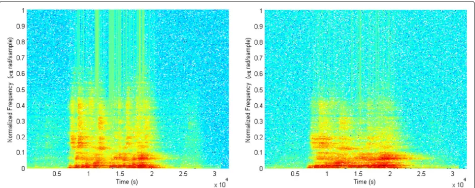
For measuring the degree of reverberation, an addi-tional feature is proposed in this paper, based on the “smearing” effect that reverberant conditions cause to the speech signal spectrogram. An example is shown in Fig.4: There, for a speech occurrence inside the bedroom of the smart home of Fig.1, the spectrograms of two sig-nals captured by a microphone located in the bedroom and one in the kitchen are depicted, showing that the latter (located outside the speech-active room) is much smoother (smeared).
To measure this effect, the proposed feature considers the signal spectrogram as a 2D image, and attempts to quantify its texture smoothness by applying to it the 2D discrete Teager energy operator of [74], yielding
m(n,t) = 2 (Sm(n,t))2− Sm(n,t−1)Sm(n,t+1) − Sm(n−1 ,t)Sm(n+1 ,t), where Sm(n,t) denotes the signal spectrogram of micro-phone m at short-time frame t ∈ T , and n is the frequency index (40-ms-long Hamming windows with a 20-ms shift and 960 frequency bins are used here). Then, as in Section5.1.3, medium-sized windowsT sliding over segmentT are considered, the time progression of which is indexed byt (600-ms-long windows with a 50-ms shift are used). The values of m(n,t) are then averaged over a part of the resulting 960×30-sized spectrogram image as:
m(t) = avg n=1,...,200
avg
t∈T{m(n,t)} ,
where the frequency domain averaging is carried out over the 200 lower frequency bins that correspond to the 0– 5 kHz frequency range of the 48-kHz sampled signal, focusing on speech content. Finally, the spectrogram tex-ture smoothness featex-ture for room r and segment T is obtained by maximizing over all room microphones and averaging the result over all medium-sized windows, namely
fr(,Tts) = avg t∈T
max m∈Mrm(
t)
Fig. 4Motivation for the spectrogram texture smoothness feature of Section5.1.4. Left: spectrogram from a microphone located inside the active speaker room (bedroom in the apartment of Fig.1). Right: spectrogram from a microphone outside it (kitchen)
5.1.5 SRP-based feature
The final feature considered for room assignment of detected speech segments is based on the steered response power (SRP-PHAT) approach of [75], and it is proposed for the first time in this paper for room-localized SAD. Employing SRP allows the creation of an acoustic map, by computing the signal power when steering microphone arrays in the direction of a spe-cific location. The position of the sound source cor-responds to that with the maximum SRP value over all possible locations. In the case of multi-room smart homes, one expects that speech originating from out-side a given room will likely exhibit high SRP values at the door region that connects that room to the rest of the apartment. In contrast, for room-inside speech, the actual source location should yield the highest SRP instead. An example for this motivation is depicted in Fig.5.
To compute the SRP-based feature for room r, a 3D region is first defined, denoted byAr that corresponds to cylindrically shaped volume(s) covering the room door(s). Specifically, on the floor plane, this lies inside room r, delineated by a 0.7-m radius semicircle around the door center, while also containing all points above it. Using a 10-cm spatial resolution for each dimension, and depend-ing on the number of doors of the room, this scheme yields approximately between 2kand 4.3kpoints, denoted as y∈ Ar, expressed in the 3D room coordinate system (see also Fig.5).
Then, for all points y ∈ Ar, the corresponding SRP-PHAT values for time frame t ∈ T are computed (200-ms-long frames with a 100-ms shift are used), by summing the generalized cross-correlations over all pairs
of adjacent microphones in room r, as:
Pr(t,y) =
(m,m) ∈ {Mr×Mr}adj
2π
0
Xm(ω,t)Xm∗(ω,t) Xm(ω,t)Xm∗(ω,t)
ejωτmm(y)dω,
where Xm(ω,t) denotes the DTFT of the mth micro-phone signal frame and τmm(y) is the time difference of arrival at pointy between the signals of adjacent micro-phonesmandm. Finally, the SRP-based feature is com-puted by summing all above values and averaging them over all windowst∈T , i.e.,
fr(,Tsrp) = avg t∈T
⎧ ⎨ ⎩
y∈Ar
Pr(t,y)
⎫ ⎬
⎭ . (8)
Clearly, the computation of this feature requires knowl-edge of the microphone topology and room layout.
5.2 Intra- and inter-room feature fusion
Using the above framework in the proposed system, for each candidate speech segment T , five features are extracted for each room r. The features are then com-bined by intra-room feature fusion (plain concatenation), resulting in five-dimensional feature vectors
fr(,allT) =
fr,(Ten), fr(,Tcoh,)fr(,Tev), fr(,Tts), fr(,Tsrp)
, (9)
for each room r=1 , 2 ,. . .,R.
Fig. 5Motivation for the SRP-based feature (the acoustic maps are shown in 2D, obtained after summing SRP-PHAT values over the
z-axis). Top: acoustic map example for speech inside the living room of the apartment of Fig.1. Middle: acoustic map example for speech outside the living room. Bottom: living room door area (two doors) employed in the SRP-based feature computation (8) for this room
•Inter-room feature concatenation, where vectors from all R rooms are concatenated, resulting in a single 5R -dimensional feature vector for segmentT ,
fhome ,(all) T = f1 ,(allT), f2 ,(allT), . . . ,fR(,allT) . (10) • Inter-room feature averaging, where vectors from each room are augmented by the feature average across the remainingR−1 rooms, resulting in ten-dimensional representations of segmentT ,
fr(, avg ,all) T =
fr(,allT), avg r=r
fr(all,T) , (11)
for each room r = 1 , 2 ,. . .,R. This way, feature vector dimensionality is no longer a function of R. Alterna-tives to (11) can also be designed, for example, employing feature extrema instead of averages.
5.3 SVM classification
The fused feature vectors are fed to appropriately designed classifiers, in order to determine the room of origin for a given segment. In this paper, linear SVMs are employed for this purpose, due to the two-class nature of the problem (inside vs. room-outside segment classification), as well as the relatively small corpus size (see also Section 7.1).1 Specifically, two SVM modeling approaches are considered, result-ing to a total of five different models, as discussed next:
• Room-specific SVM models, where a separate clas-sifier is built for each smart home room. Each training segment thus provides data to a total of R SVMs as a room-inside or -outside class sample, while during test-ing, a candidate segment is fed to the SVM of the room in which it was detected by the first stage. The SVMs can be built on any of the three feature vectors of Section5.2, given by (9), (10), or (11), thus resulting in three different systems.
•Global SVM models, where a single SVM is developed being applicable to all rooms, thus removing dependence of the number of SVM models on R. Each training segment provides its data to the global SVM a total of R times (once as a room-inside sample and R −
1 times as a room-outside one). During testing, candi-date segments are fed to this global SVM. In both cases, room-dependent features are used, provided by (9) or (11), yielding two different systems. Features (10) are not used, as they would have re-introduced dependency on R.
Among the above modeling options, the proposed sys-tem employs room-specific SVMs on inter-room con-catenated features (10). Note also that since each room
1All SVMs are trained inMatlab, by itssvmtrain.mfunction. By
decides for its own final segments, it is possible that a seg-ment gets assigned to multiple rooms or to no rooms at all.
5.4 Temporal operation and post-processing
In practice, the SVM classification of speech segments can be performed at two different temporal scales:
•Over the entire segment, where a single scalar feature is extracted for the segment for each of the five categories of Section5.1, providing a single sample for SVM training or testing. Thus, assignment to a given room is made for the whole segment.
• Over segment sliding windows, where features are extracted on medium-sized windows sliding over the given segment. As a result, each segment provides mul-tiple data points for SVM training or testing (per win-dow). The scheme allows segment breakup and selective assignment of its parts into the room that it was detected in by the first stage of the algorithm.
The proposed room-localized SAD system employs the sliding window approach, using windows of 600 ms in size advancing by a 100-ms shift. This necessitates minor modifications to the feature extraction methodology of Section5.1. In particular, there is no longer the need of averaging in (6) and (7), since the medium-sized win-dow sizes coincide, thus trivially allowing for one winwin-dow only. Further, in (4), the non-speech energy is computed over the 0.5-s interval preceding the first window of the segment.
As a final step, post-processing is also applied to the results. Specifically, speech segments with less than 0.7-s distance between them are unified, whereas speech segments of less than 0.4-s duration are deleted.
6 Baseline approaches
Two additional, simpler systems are presented in this section, both following a two-stage architecture, to serve as baselines against the developed room-localized SAD system. The first method employs MFCC features and GMM classifiers in both its algorithmic stages, while the second extends the well-known statistical model-based approach of Sohn et al. [36] to room-localized SAD, by incorporating a simple SNR-based room assignment cri-terion. Details follow.
6.1 MFCC/GMM-based system
This baseline follows our earlier work [33], and it is mainly considered in order to evaluate a system based entirely on a standard acoustic front-end (MFCC features), aiming also to demonstrate the value of the room discriminant features of Section5.1.
Its first stage is identical to that of the proposed system. Namely, for every smart home room, it performs weighted log-likelihood summation of MFCC/GMM-based scores
by means of (1) and (2) over all room microphones (M= Mr) for classes J={spr, silall} (see also Section4.4).
At the second stage, segments generated by the first stage are further examined and classified as room-inside or room-outside speech. For this purpose, room-specific GMMs are trained for each class J = {spr, spr¯}, and unweighted log-likelihood summation of MFCC/GMM-based scores is performed over all room microphones (M = Mr), followed by averaging over all short-time frames in the segment. Segments classified as room-outside speech are then deleted from the SAD output of the given room.
6.2 Sohn’s algorithm with SNR criterion
The first stage of this baseline employs the well-known and effective SAD algorithm of Sohn et al. As they detail in [36], the method is based on a likelihood ratio test between speech and noise models, considered as Gaussians in the frequency domain under an i.i.d. assumption in fre-quency and that of additive uncorrelated noise. Following noise model estimation using observed noise and of the necessary SNRs by a decision-directed approach, the likelihood ratio test is performed, and decision results are smoothed by means of an HMM-based hangover scheme [36].
In the designed baseline, Sohn’s SAD is employed for each smart home room r, using a single ad hoc selected room microphone m ∈ Mr. Then, at the second stage, for a first-stage generated segment in room r, the SNR of microphone m is compared to a global threshold; if below it, the particular segment is deleted from the room’s SAD output. This baseline thus presents a well-established and relatively simple to implement approach for room-localized SAD.
7 Databases and experimental framework
We now proceed to describe the databases where the proposed system, its variations, and baselines are eval-uated, as well as to discuss the adopted experimental framework and evaluation metrics used. In particular, the presentation refers to the experiments of Sections 8.1– 8.4. An additional dataset and a slightly modified eval-uation framework, necessary to allow comparisons with recent deep learning-based works, are detailed in the corresponding Section8.5.
7.1 The DIRHA corpora
The experiments in Sections 8.1–8.4 are conducted on two databases: the Greek-language part of DIRHA-simcorpora II [61], hereafter referred to as “DIRHA-sim”, and the “DIRHA-real” Greek corpus [16].2 The datasets are either simulated or recorded inside a smart
2DIRHA-sim is found athttps://dirha.fbk.eu/simcorpora, whereas
home apartment (with an average reverberation time of 0.72 s), developed for the purposes of the DIRHA research project [10]. Its floor plan is depicted in Figs. 1 and6, showing that five of its rooms (living room, kitchen, bathroom, corridor, and bedroom) are equipped with a total of 40 microphones grouped in 14 arrays. Most arrays consist of two or three microphones (with lin-ear topology) located on the room walls, while, for each of the living room and kitchen, a six-element pentagon-shaped array is also located at the ceiling. As a result, concerning the set of adjacent microphone pairs used in Sections 5.1.2and5.1.5, the two-element arrays pro-vide one such pair, the three-element arrays two, and the pentagon-shaped arrays five, with all latter pairs con-taining the central array microphone. The corridor thus yields the least pairs (one), while the living room the most (ten).
As indicated by its name, the DIRHA-sim dataset con-tains audio simulations, produced as detailed in [61]. Briefly, first, about 9kroom impulse responses are mea-sured at each of 40 smart home microphones from 57 pos-sible source locations uniformly distributed in the rooms of interest and with up to 8 source orientations for each (as shown in Fig.6). These are then used to convolve high-quality, close-talk speech by 20 subjects (recorded at a 48-kHz sampling rate and an SNR average of 50 dB), while real, long-duration background noises and shorter acous-tic events are also added to the resulting simulations. In total, 150 1-min simulation sequences containing speech and noise are available. In contrast, the DIRHA-real set
Fig. 6Floor plan of the multi-room DIRHA apartment where the datasets of Section7.1are simulated or recorded. Black circles indicate the 40 microphones installed inside five rooms on their walls or ceiling. Colored squares and arrows indicate possible positions and orientations of speech and other acoustic event sources (figure from [62])
contains actual recordings of 5 subjects acquired by the 40 microphones inside the smart home under realistic noise conditions [16]. In total, 60 1-min recorded sequences of speech and noise are available. Statistics of the two sets are summarized in Table1.
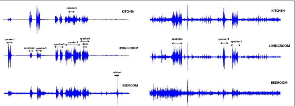
Apart from the main difference concerning the nature of the two sets (simulated vs. real), there exist two addi-tional variations, as can be also observed in the waveform examples of Fig.7. First, DIRHA-sim is characterized by more adverse noise conditions, containing more back-ground noises and acoustic events besides speech. Fur-ther, in DIRHA-sim, speech often overlaps with other acoustic events or speech in different rooms of the smart home. Indeed, as listed in Table1, speech overlap there reaches 47% (22 out of 47 min). These facts deem DIRHA-sim much more challenging for room-localized SAD than DIRHA-real.
7.2 Experimental framework and metrics
In the experiments of Sections8.1–8.4, the DIRHA-sim dataset of 150 simulations is partitioned into a train-ing set containtrain-ing 75 of them and a test set with the remaining 75. Optimization of the first-stage algorithmic parameters of Section4.3(i.e., the transition penalty and constant prior added to the speech-class log-likelihood), as well as of the global threshold used in conjunction with Sohn’s baseline, are performed on the training set. In the case of DIRHA-real, all 60 recordings are used for test-ing systems developed on the DIRHA-sim traintest-ing data. This framework allows to also gauge the usefulness of simulated databases for training models and developing features and systems that can perform well in real-case scenarios, even when differences between the sets are significant.
For evaluation, the recall, precision, andF-score met-rics are used, all computed at the frame level with a 10-ms time resolution and reported in percentage. Evaluation of room-localized SAD differs somewhat to the traditional room-independent case, as can be easily inferred from
Table 1Characteristics and statistics of the DIRHA-sim and
DIRHA-real corpora, used in the experiments of this paper
Data Databases
characteristics DIRHA-sim DIRHA-real
Speech source Loudspeaker Human
1-min-long sequences (#) 150 60
Total speech (min) 47 19
Overlapped speech (min) 22 0
Non-speech events (#) 72 Untranscribed
Background noises (#) 10 Untranscribed
Subjects (#) 20 5
Fig. 7Examples of multi-microphone data of the DIRHA corpora used in this work. Microphone waveforms in three rooms are shown. Left: a multi-speaker acoustic scene in the DIRHA-sim dataset. Right: a single-speaker scene in the DIRHA-real data
Fig. 1. In traditional SAD, the aim is to detect speech anywhere in the smart home, and as a result, each test-set sequence is evaluated only once (75 sequences for DIRHA-sim and 60 for DIRHA-real). In contrast, in the room-localized case, for each sequence, a total of R =
5 SAD outputs are evaluated (one for each room), with ground truth each time considering only speech occur-ring inside the given room. Thus, 75 × 5 = 375 and 60× 5 = 300 SAD outputs in total are evaluated for the DIRHA-sim and DIRHA-real test sets, respectively. This affects the evaluation metrics: for example, recall for room-localized SAD is computed as the ratio between the number of correctly detected room-inside speech frames and the total number of such frames in the ground truth. In total, the test set contains 447 room-inside and 1788 room-outside speech segments in the DIRHA-sim case, and 232 and 928 segments, respectively, in DIRHA-real.
8 Experimental results
Next, we report our experiments. We first focus on room-independent SAD results, subsequently covering the room-localized case extensively. We also provide an error analysis of the proposed system, as well as a study on its robustness to the number of available microphones. We conclude the section with a comparison to recent deep learning-based approaches.
8.1 Room-independent SAD
Room-independent SAD is evaluated first, primarily to showcase its easier nature compared to the room-localized task, as well as to benchmark differences between the various techniques of Sections4and6and simple channel selection schemes. Results are reported in Table2for both DIRHA-sim and DIRHA-real sets in terms of recall, precision, andF-score.
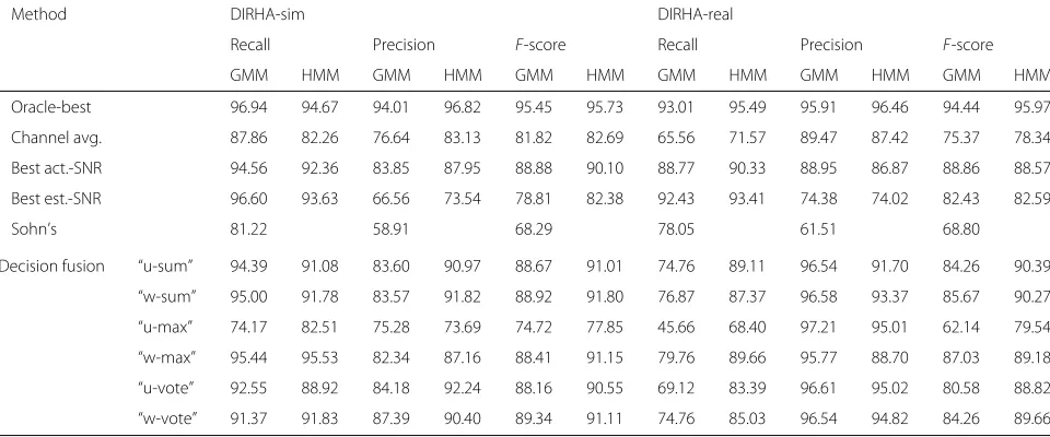
Specifically, in the lower part of Table 2, both the GMM- and HMM-based decoding schemes of Section4.3 are presented in conjunction with the six fusion tech-niques of Section 4.2, but for the room-independent SAD system variant discussed at the end of Section 4.4 that uses all 40 smart home microphones (M = Mall and J = {spall, silall}). These results are compared to two single-channel systems where microphone selection is driven by the best SNR per test-set sequence (actual based on ground-truth segmentation, or estimated), as well as the oracle-best channel result (that with the max-imumF-score per sequence) and the average of all chan-nel results. Finally, Sohn’s algorithm is also considered, applied for each room (a single room microphone is used for each room), with the union of the results across rooms obtained.
For DIRHA-sim (left side of Table2), we immediately observe the superiority of HMM-based Viterbi decod-ing over frame-based GMM segmentation. The best result is obtained by multi-channel fusion using log-likelihood summation scheme “w-sum”, achieving anF -score of 91.80%. This is significantly higher than Sohn’s method (68.29%), and it represents a 53.5% relative error reduction in F-score compared to the best estimated SNR single-channel system (91.80% vs. 82.38%). Note that the latter performs similarly to the average of all channel results (82.69%), while it lags the ideal actual SNR case (90.10%) where channel SNR computations employ ground-truth information. These comparisons confirm that the challenging nature of DIRHA-sim adversely affects SNR estimation. Note finally that the best multi-channel system still lags the oracle-best channel one (95.73%), showing potential for further improvements.
log-Table 2Room-independent SAD results on the DIRHA-sim (left) and DIRHA-real (right) test sets, further discussed in Section8.1
Method DIRHA-sim DIRHA-real
Recall Precision F-score Recall Precision F-score
GMM HMM GMM HMM GMM HMM GMM HMM GMM HMM GMM HMM
Oracle-best 96.94 94.67 94.01 96.82 95.45 95.73 93.01 95.49 95.91 96.46 94.44 95.97
Channel avg. 87.86 82.26 76.64 83.13 81.82 82.69 65.56 71.57 89.47 87.42 75.37 78.34
Best act.-SNR 94.56 92.36 83.85 87.95 88.88 90.10 88.77 90.33 88.95 86.87 88.86 88.57
Best est.-SNR 96.60 93.63 66.56 73.54 78.81 82.38 92.43 93.41 74.38 74.02 82.43 82.59
Sohn’s 81.22 58.91 68.29 78.05 61.51 68.80
Decision fusion “u-sum” 94.39 91.08 83.60 90.97 88.67 91.01 74.76 89.11 96.54 91.70 84.26 90.39
“w-sum” 95.00 91.78 83.57 91.82 88.92 91.80 76.87 87.37 96.58 93.37 85.67 90.27
“u-max” 74.17 82.51 75.28 73.69 74.72 77.85 45.66 68.40 97.21 95.01 62.14 79.54
“w-max” 95.44 95.53 82.34 87.16 88.41 91.15 79.76 89.66 95.77 88.70 87.03 89.18
“u-vote” 92.55 88.92 84.18 92.24 88.16 90.55 69.12 83.39 96.61 95.02 80.58 88.82
“w-vote” 91.37 91.83 87.39 90.40 89.34 91.11 74.76 85.03 96.54 94.82 84.26 89.66
likelihood summation, with scheme “u-sum” reaching an
F-score of 90.39%. This corresponds to a 44.8% relative
F-score error reduction compared to the best estimated SNR single-channel system (90.39% vs. 82.59%). The latter performs now better than the average of all channel results (78.34%), and it lies somewhat closer to the best actual SNR system (88.57%) than in the DIRHA-sim case, due to the less adverse DIRHA-real environment. Note finally that, as above, the best multi-channel system lags the oracle-best channel result (95.97%).
8.2 Room-localized SAD results
We now switch focus to the room-localized SAD task. Our experiments are organized as follows: First, we eval-uate the several possible choices of the system’s first stage discussed in Section 4.4. Next, we investigate its sec-ond stage and the performance of the room discriminant features of Section 5.1. Finally, we present comparative results between our proposed system and the alternative baselines of Section6.
The first experiment, reported in Table 3, compares the various design choices concerning the possible classes
Table 3Effect of the various choices in the design of the
system’s first stage (discussed in Section4.4) to the room-localized SAD performance on the DIRHA-sim test set
Oper M ClassesJ Recall Precision F-score
RI Mall {spall, silall} 72.30 56.63 63.51
RL Mr {spr, silall} 72.07 61.08 66.12
{spr, silr} 71.20 60.39 65.35
{spr, sp¯r, silall} 71.00 62.40 66.43
For consistency, the first stage is always followed by the second stage of the MFCC/GMM baseline of Section6.1. RI denotes room-independent operation (“oper”) of the first stage and RL room-localized one
and microphones used in the first stage of the room-localized SAD system, as summarized in Section 4.4. In all cases, decision fusion by means of log-likelihood summation scheme “u-sum” is employed across micro-phones. For consistency in the comparisons, the various first stages considered are always followed by an identical second stage, namely that of the MFCC/GMM baseline of Section6.1.
It is clear from Table 3 that the room-independent scheme leads to the worst performance, trailing all room-localized variants. The basic reason is that in the lat-ter schemes, the first stage can achieve high recall for room-inside speech and produces less room-outside seg-ments compared to the room-independent case; thus, the second stage has an easier task. The second line of the table corresponds to the classes and microphone set options chosen in the proposed system. These yield the highest recall (72.07%) among the room-localized SAD variants, with an F-score second, but very close, to the three-class modeling approach of the last line (66.12% vs. 66.43%).
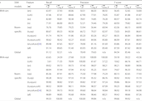
The second experiment, reported in Table 4, con-centrates on the proposed room discriminant features of Section 5.1, as well as their feature fusion schemes of Section 5.2 and the SVM modeling approaches of Section5.3 operating over entire segments. The evalua-tion is conducted for the room-inside vs. room-outside speech classification task of the second stage of the developed algorithm. For this purpose, the ground-truth speech boundaries are used, thus decoupling the com-parisons from the first stage. Further, results include four rooms of the smart home, excluding the corridor (R =
Table 4Performance of the room discriminant features of Section5.1and their combinations, in conjunction with inter-room fusion (Section5.2) and SVM modeling (Section5.3) for the room-inside vs. room-outside speech classification task of the second stage of the proposed algorithm
Set SVM Feature Recall Precision F-score
models (•) fr(,•T) fr(, avg ,•) T fhome ,(•) T fr(,T•) fr(, avg ,•) T fhome ,(•) T fr(,•T) fr(, avg ,•) T fhome ,(•) T
DIRHA-sim (en) 63.97 37.93 40.06 50.51 86.03 86.92 56.45 52.65 54.84
(coh) 47.46 87.41 88.66 67.90 77.01 76.05 55.87 81.88 81.87
(ev) 82.89 90.81 90.38 78.01 74.85 76.28 80.37 82.06 82.74
(ts) 71.91 86.00 89.35 52.21 74.46 79.28 60.50 79.82 84.01
Room- (srp) 76.76 79.85 79.25 53.94 56.44 60.94 63.36 66.13 68.90
specific (ts,srp) 80.67 89.33 90.58 66.72 79.37 82.97 73.03 84.05 86.61
(ts,srp,ev) 91.74 90.74 91.86 85.20 83.26 85.27 88.35 86.84 88.44
(ts,srp,ev,coh) 90.62 90.42 92.27 83.65 84.96 85.80 86.99 87.61 88.92
(en,coh,ev)[34] 89.48 87.65 90.37 78.90 81.16 81.69 83.86 84.28 85.81
(all) 91.14 89.65 91.40 83.93 85.30 85.40 87.39 87.42 88.30
Global 91.12 92.21 n/a 78.49 79.63 n/a 84.34 85.46 n/a
DIRHA-real (en) 63.65 24.39 27.68 55.30 100.00 100.00 59.18 39.22 43.36
(coh) 5.61 71.35 78.99 100.00 61.67 57.22 10.62 66.16 66.71
(ev) 99.02 99.73 99.73 97.40 98.07 98.21 98.21 98.89 98.96
(ts) 68.94 97.44 97.94 81.42 95.25 93.41 74.67 96.33 95.62
Room- (srp) 85.36 87.91 80.75 75.50 77.98 75.29 80.13 82.65 77.93
specific (ts,srp) 90.28 94.52 97.33 91.58 95.32 86.76 90.92 94.92 91.74
(ts,srp,ev) 99.90 98.82 97.81 99.82 97.87 97.24 99.86 98.34 97.53
(ts,srp,ev,coh) 98.52 98.99 98.11 99.94 98.37 87.09 99.23 98.68 92.27
(en,coh,ev)[34] 98.25 99.73 99.50 99.60 98.64 90.84 98.92 99.18 94.98
(all) 98.89 98.85 95.68 99.94 98.46 80.21 99.42 98.66 87.26
Global 99.33 100.00 n/a 100.00 99.84 n/a 99.66 99.92 n/a
Results are reported onR=4 rooms of the DIRHA smart home (excluding the corridor) on the DIRHA-sim (top) and DIRHA-real (bottom) test sets using ground-truth speech segment boundaries. All SVMs operate over entire segments
and four feature combinations are listed, as selected by wrapper-based sequential forward feature selection [76, ch. 5.7.2] that is conducted on DIRHA-sim (based on the corresponding proposed system F-scores). In addition, the three-feature subset of our previous work [34] is eval-uated. Notice that the notation in (10) and (11) is slightly extended to allow inter-room fusion of single features and subsets.
Concerning DIRHA-sim (Table4, top), in the case of room-specific SVMs, we observe that for most individ-ual features of Section 5.1 (with the exception of the energy-based one), performance improves by inter-room fusion. The best feature is the proposed spectrogram tex-ture smoothness, achieving an F-score of 84.01% after fusion by (10). In contrast, the energy-based feature per-forms the worst at a 52.65%F-score after fusion by (11). For the entire feature vector (“all”) obtained by intra-room fusion (9), small differences are observed between no room combination and inter-room fusion by (10) or
(11), with the bestF-score reaching 88.30%. Global SVM modeling performs slightly worse (85.46% F-score with fusion (11)).
Regarding feature subsets, the best two-feature set con-sists of the spectrogram texture smoothness and the SRP-based feature; envelope variance is then added to yield the best three-member set; and subsequently, the coherence-based one is chosen. All subsets demonstrate better per-formance than individual features, when fused by (10) or (11). Also, we can observe that energy does not boost performance further, as the best four-feature set slightly outperforms the “all” set, achieving an 88.92% vs. 88.30%
F-score with fusion (10). Finally, compared to our previ-ous work [34], the “all” set achieves a 17.5% relative error reduction inF-score (88.30% vs. 85.81% with (10)).
DIRHA-sim) and SRP-based ones fail to do so. The highest performing feature is the envelope variance with an
F-score of 98.96% after fusion by (10), closely followed by spectrogram texture smoothness at 96.33% after fusion by (11). For the entire feature vector (“all”) obtained by intra-room fusion (9), small differences are observed between no room combination and inter-room fusion by (11), regardless of the SVM models used. However, concatenation across all rooms by (10) fails to improve matters (an F-score of only 87.26% is attained). This is probably due to the high dimensionality of the result-ing vector and the use of multiple SVMs, in conjunc-tion with the mismatch between the DIRHA-sim trained models and DIRHA-real test conditions. This seems also supported by the fact that inter-room fusion by means of (11) in most cases outperforms (10). Never-theless, the best “all” feature system reaches an almost perfectF-score of 99.92%, obtained by global SVMs and fusion (11). Note also that this is very close to the 99.86%F-score of the spectrogram texture smoothness-SRP-envelope variance combination with no inter-room fusion.
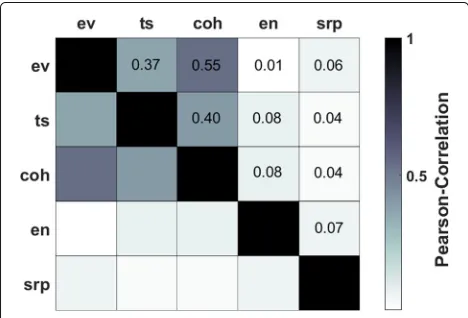
As a complement to this experiment and to further gain insights into the room discriminant features, their lation is investigated. For this purpose, the Pearson corre-lation coefficient is computed among all features over the speech segments of the DIRHA-sim test set, resulting in the matrix of Fig.8. As expected, the envelope variance, spectrogram texture smoothness, and coherence-based features demonstrate high correlation between them, as they are all related to reverberation. On the contrary, the energy- and SRP-based ones exhibit low correlation with all features.
In the third experiment, reported in Table5, once again ground-truth segments are considered as input to the
Fig. 8Pearson correlation coefficients between the room discriminant features of Section5.1, computed on DIRHA-sim (ev, envelope variance; ts, spectrogram texture smoothness; coh, coherence-based; en, energy-based; srp, SRP-based)
second stage. The aim here is threefold: first, to showcase the superiority of the proposed room discriminant feature approach over the baselines of Section6; second, to high-light performance differences among the various smart home rooms; and third, to further compare the fusion schemes of Section 5.2. Specifically, the MFCC/GMM-based second stage of the baseline of Section6.1is listed in the first line of Table 5, followed by the SNR-based room assignment scheme of Section6.2, as well as room-specific SVM modeling on (9), (11), and (10) operating over entire segments.F-scores are reported for each room separately (no corridor F-score is shown for DIRHA-real, as there are no ground-truth room-inside segments there), as well as for all four (excluding the corridor) or five rooms.
It is clear from Table5that the proposed approach dra-matically outperforms the baselines, e.g., for R= 5, on DIRHA-sim, the best result (84.26%) represents a 46.7% and 73.2% relative error reduction over the baselines of Sections6.1and6.2, respectively, while on DIRHA-real, the corresponding reductions of the best result (93.34%) stand at 78.6% and 87.8% relative. It is also clear that the corridor is a challenging room, as seen by its low DIRHA-simF-scores and the performance drop from the
R = 4 to the R = 5 case. This is primarily due to its central location in the smart home floor plan (see also Fig. 6) exposing it to sounds coming from all other rooms, as well as the small number of microphones in it (only two). Regarding the multi-room results of the fea-ture fusion schemes of Section 5.2, inter-room feature concatenation (10) performs best on DIRHA-sim, fol-lowed by (11). This can be expected as (10) captures more detailed information (albeit at higher dimension-ality). Similarly, fusion (11) is superior to the lack of inter-room combination in (9). On DIRHA-real, how-ever, the above are reversed, as features (9) outperform (11) and, in turn, fusion by (10). This is primarily due to the mismatch of the DIRHA-sim trained SVMs to the DIRHA-real conditions, thus favoring lower-dimensional representations that generalize better, as also observed in Table4.
Finally, Table 6 reports on the full task of room-localized SAD. Its upper part covers single-stage methods, namely the best room-independent approach (“best RI”), as well as the first stages of the MFCC/GMM baseline of Section 6.1(recall that this is identical to the proposed system’s first stage) and Sohn’s algorithm (Section 6.2). The complete two-stage baselines are evaluated next, followed by the proposed algorithm employing room-specific SVMs on features (10) operating over the entire segments (“seg”) or over sliding windows (“win”), where results both with and without the corridor are reported.