R E S E A R C H A R T I C L E
Open Access
Realization of CAD-integrated shell
simulation based on isogeometric B-Rep
analysis
T. Teschemacher
1*, A. M. Bauer
1, T. Oberbichler
1, M. Breitenberger
1, R. Rossi
2, R. Wüchner
1and
K.-U. Bletzinger
1*Correspondence:
1Lehrstuhl für Statik, Technische
Universität München, Arcisstr. 21, 80333 Munich, Germany Full list of author information is available at the end of the article
Abstract
An entire design-through-analysis workflow solution for isogeometric B-Rep analysis (IBRA), including both the interface to existing CADs and the analysis procedure, is presented. Possible approaches are elaborated for the full scope of structural analysis solvers ranging from low to high isogeometric simulation fidelity. This is based on a systematic investigation of solver designs suitable for IBRA. A theoretically ideal IBRA solver has all CAD capabilities and information accessible at any point, however, realistic scenarios typically do not allow this level of information. Even a classical FE solver can be included in the CAD-integrated workflow, which is achieved by a newly proposedmeshlessapproach. This simple solution eases the implementation of the solver backend. The interface to the CAD is modularized by defining a database, which provides IO capabilities on the base of a standardized data exchange format. Such database is designed to store not only geometrical quantities but also all the numerical information needed to realize the computations. This feature allows its use also in codes which do not provide full isogeometric geometrical handling capabilities. The rough geometry information for computation is enhanced with the boundary topology information which implies trimming and coupling of NURBS-based entities. This direct use of multi-patch trimmed CAD geometries follows the principle of embedding objects into a background parametrization. Consequently, redefinition and meshing of geometry is avoided. Several examples from illustrative cases to industrial problems are provided to demonstrate the application of the proposed approach and to explain in detail the proposed exchange formats.
Keywords: Isogeometric B-Rep analysis, IBRA, IGA, Exchange format, Computer-aided design, CAD, CAD-integrated analysis, Design-through-analysis workflow
Introduction
The possibility of bridging the gap between CAD and computational models drove over
the last years the development of “Isogeometric” approaches (as shown in Fig.1). Such
techniques, which employ directly the NURBS discretization in the computational pro-cess, proved very successful in addressing a variety of problems thanks to the excellent mathematical properties of the NURBS basis.
©The Author(s) 2018. This article is distributed under the terms of the Creative Commons Attribution 4.0 International License (http://creativecommons.org/licenses/by/4.0/), which permits unrestricted use, distribution, and reproduction in any medium, provided you give appropriate credit to the original author(s) and the source, provide a link to the Creative Commons license, and indicate if changes were made.
Fig. 1 The gap between CAD and computational models. The desired work flow from CAD to CAD is displayed here. Geometries which are used for design in CAD will be the bases for numerical models during the analysis in the solver. Finally, the original geometry will used for the processing of the upcoming solutions of the computations
Unfortunately, the direct use of general CAD models in the computational process turned out to be very demanding and is to date not yet fulfilled. The key to the outstand-ing difficulties can be found in the pervasive use of “trimmoutstand-ing”, a technology by which some parts of the domain can be excluded from the model by prescribing their shape within the parametric discretization of a regular quadrilateral NURBS. Moreover, the usage of trim-ming requires the description of the topology (e.g. connectivity of patches) of CAD models, usually given by a boundary representation (B-Rep). Thus NURBS-based B-Rep models are the standard model description within CAD systems for practical engineering problems. While the idea of NURBS-based B-Rep models and the modelling with them is con-ceptually intuitive and is very mature within CADs, including such capability within a computational model is far from trivial, since the introduction of trimming lines breaks the continuity of the shape functions employed in the calculation [1]. A number of dif-ferent research lines, oriented to the solution of such problem were presented over the
years. For example, the use of T-Splines [2,3] allows sidestepping the difficulty by
pro-viding a way to mesh complex surfaces without having to use the trimming technology. Even though such technique has been partially successful, it relies on a user-driven mesh cleaning step, and hence does not constitute a viable solution in the challenge of using unmodified CAD data.
More recently, the introduction of the isogeometric B-Rep analysis (IBRA) technology [1,4] provided a novel approach to address the challenge. The idea leveraged by IBRA is to keep using all control points included in the model, considering however that only a portion of the domain, the one enclosed by trimming lines, is actually considered in the computational structural analysis, more specifically in the integration process. Such an approach employs the fundamental idea of “Embedded techniques” in which objects are enclosed within a non-matching computational domain enabling the application of boundary conditions at arbitrary positions within the computational domain.
and can be performed in different ways, for example by a penalty approach [4] but also by employing Lagrange multipliers [5,6] or Nitsche-type methods [5]. In a broad sense,
CutFEM [7] and finite cell [8,9] approaches can be considered as variations of such idea.
In the practice, achieving a convenient implementation of such model poses important challenges, since it does not fit well with the traditional finite element workflow. The pur-pose of the current paper is therefore twofold: firstly the bandwidth of possible realizations of the IBRA technology with suitable solver designs is described, secondly an integrated approach to the whole computational pipeline, i.e. from CAD to computation, is defined for the different levels of isogeometric fidelity in the structural solvers.
A theoretically ideal IBRA solver has all CAD capabilities and information accessible at any point, which is not achievable in realistic scenarios. Therefore, variants of optimally CAD-integrated solvers need to be elaborated with distinct CAD-related functionality which results in different type and amount of data at the interface between CAD and structural analysis. As the other extreme, even a classical FE solver can be included in the
CAD-integrated workflow, which is achieved by a newmeshlessapproach. This facilitates
significantly the implementation of the IBRA approach in any solver. To this end, the key observation is that the implementation of IBRA (or of any FEM-type calculation) on the level of assembly only relies on the knowledge of shape functions, shape function deriva-tives and integration weights at the integration points. Once such information is available, each integration point can be treated as an independent “element” connecting the “cloud” of control points whose shape functions are non-zero at the integration point position.
The advantage is that the integration points do not need to be located according to a regular tensor-product based structure, thus naturally fitting the need of covering an irregularly trimmed domain homogeneously.
Following this idea, the paper addresses in detail how multiple patches as well as trim-ming lines and coupling information can be conveniently treated in the framework of the proposed approach. This is levering the idea that the support (read as “cloud” or relevant control points) of integration points located at the domain interfaces (trimming lines or patch boundaries) can naturally span multiple domains. This approach thus allows decou-pling the calculations between a geometrical kernel, in charge of generating suitable inte-gration points, identifying the relevant clouds of control points and computing the shape functions, and a computational kernel completely agnostic to such geometric operations. Our claim is that this naturally defines a computational pipeline from CAD to calcula-tion (and eventually back to CAD), which can be decomposed in modules, each largely independent of the others. A group may then decide to address the complete pipeline or to focus on some of the rings of the chain, be it in the geometrical decomposition or the computational back end, the same way as it is normally done in the FEM commu-nity (meshing and computation) but without losing the advantage of preserving the exact geometry and the advantages of the NURBS basis through the entire pipeline.
data needed for the mentionedmeshlessapproach, thus dumping to disk and reloading when needed the control point cloud as well as all the information needed to perform calculations.
From a formal point of view, the structure of the paper is as follows:
• “Isogeometric B-Rep analysis (IBRA)” section summarizes briefly the main aspects
and components as well as the required notation for IBRA.
• “Solver design” section investigates systematically the possible solver designs suitable
for IBRA.
• “Design-through-analysis workflow” section identifies the required
CAD–CAE-coupling data and defines data interfaces for the IBRA design-through-analysis work-flow.
• “IBRA exchange format” section elaborates exchange formats for the necessary data
interfaces which eventually enable the IBRA workflow for complex geometry models.
– “Data interface—Geometry” section explains the geometrical description of sur-face models including their topologies.
– “Data interface—Integration domains” section describes the corresponding inte-gration domains.
– In “Data interface—Integration points” section a possible data exchange on level
of integration points i.e. themeshlessintegration points is shown.
• “Simulation of real CAD models” section demonstrates with some advanced structural
analysis problems based on real-world CAD models that the presented workflow is working successfully.
• “Conclusion” section summarizes the document and gives an outlook to further
research.
• Appendix A provides some basic and precisely documented examples for a better
understanding of the proposed format for the geometries (corresponding to “ID sys-tems” and “Data interface—Geometry” sections).
• Appendix B contains some well-documented examples for a better understanding
of the proposed format for the integration domains (corresponding to “Integration domains within IBRA” and “Data interface—Integration domains” sections).
Isogeometric B-Rep analysis (IBRA)
Isogeometric B-Rep analysis[4] can be seen as an extension of theisogeometric analysis
(IGA). IBRA uses in addition to the basis functions from CAD, the Boundary
Repre-sentation (B-Rep, see also “Boundary representation (B-Rep)” section) description for approximating solution fields. Thus, it allows to analyze thin-walled structures directly based on the CAD model.
NURBS-based B-Rep models
V1
˜(7)
( ˜ξ)
˜(3)
( ˜ξ)
˜(1)( ˜ξ) ˜(6)
( ˜ξ) ˜(5)
( ˜ξ)
˜(4)
( ˜ξ)
(2)( ˜ξ) (1)( ˜ξ)
(2)( ˜ξ) (3)( ˜ξ)
(4)( ˜ξ) (5)( ˜ξ)
(6)( ˜ξ)
(7)( ˜ξ)
(1) (ξ,η)
1
6 5
4 3
2 7
2 4
3 5 6
7,8
˜
D(1)
D
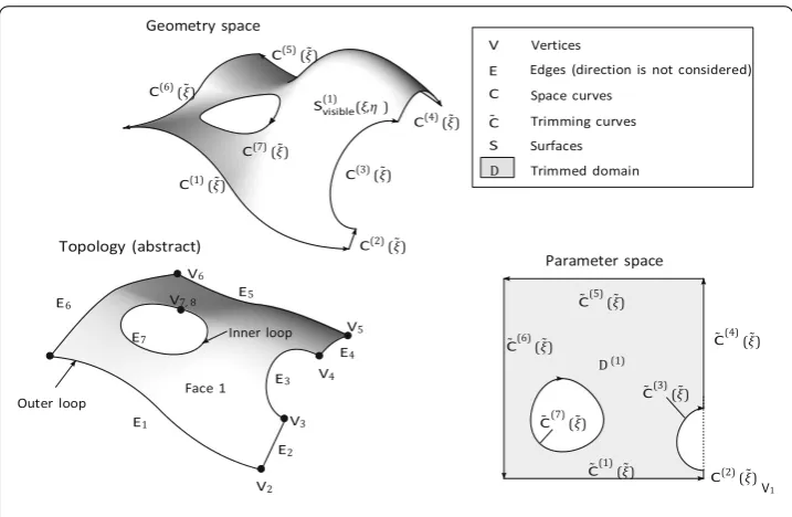
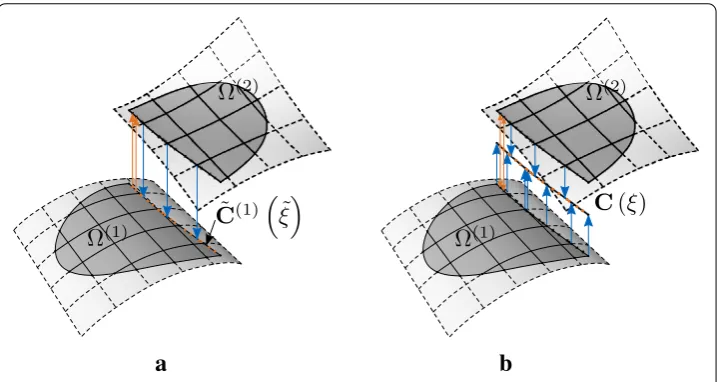
Fig. 2 Example of B-Rep surface (trimmed surface) withinGeometryandParameter spaceincluding its Topology. The surfaceS(1)visible(ξ,η) is bounded by the trimming curves ˜C( ˜ξ) resp. space curvesC( ˜ξ) within the parameter resp. geometry space (modified figure from [4])
Boundary representation (B-Rep)
In geometric modelling, B-Rep is a method for representing shapes using boundaries. The boundary representation of an object consist of two parts:
• Geometry (shape), which defines the spatial position, curvatures, etc.
• Topology, which allows to make links between geometrical entities.
The three main topology entities are
• Faces.
• Edges.
• Vertices.
Thus, a solid for example is defined by a set of enclosing surfaces, namedfaces. Those
faces are bounded byedges(E) lying on the surface. These edges are geometrically
rep-resented by curves. Finally, the curves are bounded by points named vertices (V). The set of curves that are enclosing the surfaces are called trimming loop. One distinguishes between inner (holes) and outer loops. Inner loops are defined clockwise and outer loops are defined counter-clockwise. An example of a B-Rep surface, i.e. a trimmed surface is
shown in Fig.2.
NURBS basis functions for curves and surfaces
B-Spline basis functions Ni,p depend on the knot vector, which is defined by a set
of non-descending parameters, and a polynomial degree p. The basis functions can be
evaluated by theCox-de Boor[14,15] recursion formula.
A geometry could be expressed by a linear combination ofnshape functions with their
respective control pointsPi. The formula for a B-Spline curveC(ξ) is given by
C(ξ)= n
i=1
Ni,p(ξ)·Pi. (1)
In contrast to that, NURBS basis functions have an additional weightwifor every control
point. The weight controls the influence of a control pointPi respectively of the
corre-sponding shape functionNi,pon the final geometry. The NURBS becomes a B-Spline if
all weights are equal. Otherwise, it leads to rational basis functions that allow the exact representation of any conic section properly (e.g. circles) which makes NURBS popular in computer-aided design.
Considering a weight for each control point leads to the formula for NURBS curves in
Eq. (2) with the corresponding basis functionsRi,p.
C(ξ)= n
i=1
Ni,p(ξ)·wi
n
j=1Nj,p(ξ)·wi Pi=
n
i=1
Ri,p(ξ)·Pi (2)
NURBS surfaces are defined by a tensor product of NURBS basis functions with the
two parametric dimensionsξandη. The corresponding geometry description for NURBS
surfaces is given by
S(ξ,η)= n
i=1 m
j=1
Ni,p(ξ)·Mj,p(η)·wij·Pij
n
k=1
m
l=1Nk,p(ξ)·Ml,p(η)·wkl
=
n
i=1 m
j=1
Rij,pq(ξ,η)Pij (3)
with pandq being the polynomial degrees andNi,p(ξ) andMj,q(η) the corresponding
independent shape functions.
Trimmed NURBS surfaces
A trimmed NURBS surface is described by a NURBS surface and a set of Mproperly
ordered boundary (trimming) curves ˜Ck(˜ξ) withk=1,. . ., Mlying within the parameter
space of the surface (see also [16]). Thus, a trimmed surface is a partially visible surface,
defined by thetrimmed domainwhich is described by the trimming curves. In general,
trimming curves can be of any form, however, when dealing with NURBS entities, it is
desirable to represent these with NURBS, too. The curves ˜Ck(˜ξ) are joined properly to
form outer and inner loops. The outer loops are oriented counter-clockwise, whereas
the inner loops are oriented clockwise (see also Fig.2). Since for geometric modeling an
explicit description of the boundary within the geometry space is needed, the trimming
curves ˜Ck(˜ξ) are mapped onto the surface as an explicit space curveCk(ξ) (see also [17]).
B-Rep edges
Edges are the second topological entity in a B-Rep model. They describe the boundaries of
the surfaces and contain furthermore topological relationships (cf. topology in Fig.2). An
η ξ
ξG
ηG
J2
J1
˜
J2
ξG
˜
ξ
˜
J1
Fig. 3 Mapping operations betweenGeometry spaceandIntegration domainfor the surface and a trimming curve, respectively (modified from [18])
given in spatial coordinates and links to the corresponding trimming curves ˜C(˜ξ) of the
adjacent faces. This information can be transferred to IBRA for coupling and boundary
conditions.
The trimming curves are analogously to space curves described as NURBS curves.
˜
C(˜ξ)= n
i=1
Ri,p(˜ξ) ˜Pi (4)
Note that, all entities with specifier ˜•refer to a parameter space of a surface.
Conse-quently, the coordinates of the control points ˜Piare given with respect toξ andηof each
NURBS surface. ˜ξdenotes the curve parameter along the trimming curves.
Integration domains within IBRA
Isogeometric B-Rep analysis requires the numerical integration of trimmed domains and
their boundaries resp.edges. The latter are needed because a strong enforcement of
bound-ary conditions is in general not possible and thus, they require a weak imposition, which eventually leads to the evaluation of an integral.
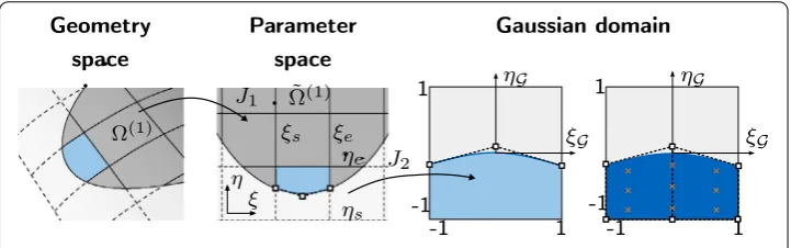
Figure3summarizes the different necessary mapping operations for surfaces and edges.
Numerical integration of surfaces
The area|A|of a trimmed surface element is defined within the parametric coordinates
ξ ∈[ξs,ξe] andη∈ [ηs,ηe]. The corresponding control points of the curve segment are
mapped into theGaussian domainGby shifting, scaling and rotating. This curve is then
used for constructing an auxiliary surface ˆSin theGaussian domain, which in return can
be integrated as a conventional untrimmed NURBS surface. More details can be found in [1].
The corresponding formula is given by
|A| =
A
dA=
ξe
ξs ηe
ηs
J1dξdη=
GJ1J2dG (5)
withGbeing theGaussian domain. In Eq. (5) the JacobianJ1represents the mapping from
GeometrytoParameter space(see Fig.3). This mapping can be derived by using the base
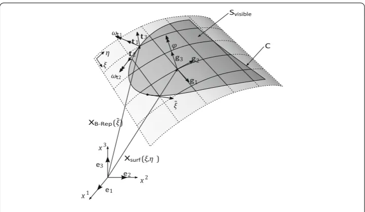
vectorsg1andg2(shown in Fig.4) as follows
x3
x2
x1 3
1 2
1 2 3
φ t2
t3
t1
η ξ
ω1
ω2
( ˜ξ)
(ξ,η) ˜ ξ
Fig. 4 B-Rep model of a trimmed surface with the respective base vectors for the surface and the edge in Geometry space
The mapping fromParameter spaceto theGaussian domainG(withξG ∈[−1,1]×ηG∈
[−1,1]) is defined as the JacobianJ2
J2= ∂ξ∂ξ G
∂η
∂ηG , (7)
whereξ andηare the parameters inParameter spaceandξG andηG the corresponding
parameters which describe theGaussian domain.
The mappingJ2is deformation independent and can thus be included in the so-called
weighting factorw˜l(see also [1]) of a quadrature pointlwhich is given by
˜
wl =J2wl (8)
withwlbeing the Gaussian quadrature weight used for integrating theGaussian domain.
With the knowledge of theweighting factorw˜lthe area of a surface can be easily
com-puted as follows
|A| ≈ nqp
l=1
J1w˜l. (9)
Numerical integration of edges
A B-Rep edge element is a segment of a NURBS curve, defined within a trimming curve of an underlying surface. The B-Rep edge element is used for distinct purposes e.g. patch coupling or imposition of Neumann and Dirichlet boundary conditions. Examples of
B-Rep edges are given in Fig.5. The length of a B-Rep edge|e|can be computed as follows
|e| =
e
de=
˜ ξ
˜
J1d˜ξ =
G ˜
J1J˜2dG, (10)
where ˜J1describes the mapping fromGeometrytoParameter spaceof the trimming curve
with its parameter ˜ξ. ˜J2represents the mapping fromParameter spaceto theGaussian
Fig. 5 Different types of B-Rep edges, e.g. for coupling of two patchescor imposition of Dirichletdand Neumannnboundary conditions
˜
J1can be evaluated as follows
˜
J1=g1·˜tξ+g2·˜tη2 , (11)
with the two base vectorsg1andg2of the surface and the components of the trimming
curve tangent given by ˜tξ = ∂ξ∂ξ˜ and ˜tη = ∂η∂ξ˜ as shown in Fig. 5. The second mapping
parameter ˜J2is defined as
˜
J2= ∂
˜ ξ
∂ξG . (12)
This ˜J2mapping is deformation independent and can thus be included analogously to the
surface integration in the so calledweighting factorw˜l(see also [1]) of a quadrature point
lgiven by
˜
wl =J˜2(˜ξ)·wl (13)
withwlbeing the Gaussian quadrature weight used for integrating theGaussian domain.
As ˜J2theweighting factorw˜lis deformation independent. Thus, it can be precomputed.
The length of a B-Rep edge can be easily computed with ˜wlas follows
|e| ≈ nqp
l=1
˜
J1w˜l. (14)
Numerical Integration Procedure
TheNumerical Integration Procedureis one of the important and challenging parts of the
IBRA workflow. During this process a properIntegration domainis defined and created.
The procedure is split to theIntegration Domainof surfaces (see “Surface integration
procedure” section) and of edges (see “Coupling edge integration procedure” section). The necessary tasks, difficulties and possible ways of the procedure are described in this section.
Surface integration procedure
IBRA evaluates element functions over trimmed NURBS surfaces by calculating
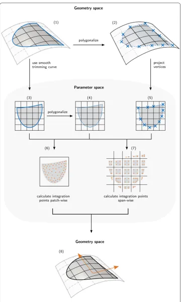
integra-tion points inside the trimmed domain. Figure6shows different approaches to define the
Fig. 7 AGIP integration procedure: sub domain of(1)(blue) in theGeometry spaceand in theParameter spacewith a segment of the refined trimming curve. Mapped sub domain and trimming curve in the Gaussian domainand auxiliary NURBS surface for the integration points
• The first step is to decide if the boundaries are approximated for a simpler computa-tion of the integracomputa-tion domains. The approximacomputa-tion can be realized by transforming the exact boundaries in geometry space (1) to a polygon (2) by mapping the vertices into the parameter space (5) or by a polygonalization of the NURBS trimming curves (3) in the parameter space (4). Doing the approximation in geometry space allows to define the tolerances for the polygonalization (max. edge length, angle deviation, etc.) in real units while using the parameter space leads to simpler 2D operations. Using the smooth boundary curve (1 and 3) leads to an exact representation of the trimming domain but also to complex geometric operations.
• The next step is the subdivision into integration domains for the computation of the integration points. Here, one can generally divide the methods in the two categories of patch-wise (6) and span-wise integration (7). Patch-wise integration has the advantage of less integration points whereas patch-wise segmentation has to deal with less trimming scenarios.
• The necessary entities in the geometry space (8) for the element formulation can finally be derived at the defined integration points.
Further literature on trimming and the achievable quality of the solutions by employing alternative approaches to the presented AGIP method by [1] in “Numerical integration of
surfaces” section, can be found in [19–26] (Fig.7).
Coupling edge integration procedure
The discretization has to be evaluated over the trimming curves of both patches to evaluate the coupling edge information. Either the geometry or the parameter curve can be used
for the discretization of theIntegration Domainat the edge (cf. Fig.8). As a consequence,
different mapping operations of knot lines and integration points become necessary. In the following the two different projection techniques will be explained briefly (see
Fig.8). One will take the parameter curve as reference, one is describing the discretization
on the geometry curve.
a. The discretization is made on the parameter curve ˜C(1)ξ˜of patch (1) (Fig.8a). The
procedure of this strategy can be as follows:
• Find all intersections of the parameter curve of patch (2) with the knots of the
a
b
Fig. 8 Derivation of the integration points for the coupling domain. The intersecting knot lines from master and slave patch are mapped to the respective coupling curve, the integration domain is derived as for a classic curve, e.g. by Gauss points, and those integration points are mapped back onto the patches.a Trimming curve of the master patch is the coupling curve.bGeometry curve is the coupling curve as also described in [27]
• Project the geometric positions of all intersections to the parameter curve
˜
C(1)ξ˜and find all intersections of the parameter curve with the knots of patch
(1).
• All intersections provide space for curves in Gaussian domain. It should be
considered the highest polynomial order of both patches.
• Take integration points on patch (1) additionally project the integration points
to theParameter spaceof patch (2) to have the position on both patches.
b. A curveC(ξ) inGeometry spacewhich represents both parameter curves is used
for discretization of the coupling curve (Fig.8b). The procedure using the geometry
curve can look as follows:
• Obtain geometry curve fitting to both parameter curves. The curve will be
already given as described in the format from “Data interface—Geometry” sec-tion.
• Find all intersections of both parameter curves with the knots of their underlying
patches, respectively.
• Project all obtained intersections to theParameter spaceof the geometry curve
C(ξ).
• In all of the upcoming spaces between the intersections are introducedGaussian
domains. The highest polynomial order of both patches is to be used here.
• Project the geometric position of all integration points to parameter space of
both patches as the position on both patches is needed.
the parameter curve only the projection to patch (2) is needed. Whilst using the geometry curve the integration points have to be projected to both patches.
Analysis-related enhancement of geometrical data
In the following the analysis-related enhancements of geometrical data is given for surface-and B-Rep edge element formulations.
Surface element formulations are used to represent the shape and solution of the phys-ical problem. Examples for element formulations of isogeometric surface elements for membranes can be found in [28,29] and for shells in [30–38].
B-Rep element formulations can be used for imposing different types of boundary con-ditions on arbitrary locations within the geometry model. In principle, the following types of boundary conditions can be enforced in a weak sense:
• Neumann boundary conditions.
• Dirichlet boundary conditions.
• Mechanically motivated, e.g. cables (Philipp et al. [29]) or beams (Bauer et al. [39]).
• Patch coupling conditions to connect distinct patches with arbitrary
parameteriza-tions.
In general, these boundary conditions have to be fulfilled along the whole edge. Note that knot lines have to be taken into consideration for accurate integration results [1].
There exist several general methods for implying Dirichlet boundary conditions. Two of them, namely
• Penalty approach,
• Lagrange multiplier method,
will be briefly outlined within the context of IBRA for enforcing continuity (coupling) between patches and imposing prescribed displacements or rotations in the following sections.
This section describes the basic principles of line-wise imposed boundary conditions
and can easily be transferred to other approaches as e.g. in [5,6,19,24,40–46].
All approaches have the integration along the edge in common, as proposed in “Numer-ical integration of edges” section.
The use of Nitsche’s technique in the imposition of interpatch-continuity also
repre-sents a common and well explored alternative [5,44,47–52]. While such option is clearly
superior to the use of simpler approaches, it is less efficient in implementation and com-putational costs, in the sense that it requires modifying the variational form as well as evaluating boundary integrals at the boundaries of interest. Thus, in the current work it is focused on the alternatives, the penalty method and the Lagrange multiplier method.
Continuity between patches
The following section explains a weakG0andG1coupling of two trimmed patches on a
B-Rep edge (see also ˜e(1)and ˜e(2)in Fig.5). Two different approaches are explained briefly
Penalty approach
Considering the virtual work termδWBpenalty−Rep along a B-Rep edge aG1continuity can be
enforced along it as follows
δWBpenalty−Rep =δWdisp+δWrot . (15)
Equation (15) contains two expressions one for coupling the displacementsδWdisp, i.e.
G0, and one for coupling the rotationsδWrot, i.e.G1, along an edge. They are given by
δWdisp= −αdisp
(1) e
u(1)−u(2)· δu(1)−δu(2) d(1)e (16)
δWrot = −αrot
(1) e
ω(1)
T2 −ω
(2) T2
· δω(1)
T2 −δω
(2) T2
d(1)e (17)
with
δω(i)
T2 =
∂ω(i) T2 ∂u(i) ·δu
(i). (18)
Hereu(1)resp.ω(1)
T2 represent the displacement resp. rotation around the tangent of the
boundary of the master patch. The index two is used for the corresponding quantities on the slave side. As the penalty factor can differ between displacements and rotations, two
distinct factors are introduced,αdispandαrot. The right choice of the penalty factor is very
important as a bad choice of the penalty factor can lead to numerical problems (see also
[4]). The additional virtual workδWBpenalty−Rep is used to account for the coupling conditions
in a weak sense. In case of matching discretizations this vanishes and the coupling is inherently satisfied.
The discrete form of Eq. (16) is given for example by
δWdisp≈αdisp· nqp
k ˜
wk˜J1k n(1)
cp
i
R(1)i (ξk(1),η(1)k )·u(1)i − n(2)cp
j
Rj(2)(ξk(2),η(2)k )·u(2)j
(19)
with ˜wkand ˜J1kbeing the weighting factor and the Jacobian for the boundary(1)as given
in Eq. (14). Exemplary integration points are shown in Fig.8.
The stiffness of the coupled system is given as follows
K=
K(1)+K(1)p C(1p,2) C(2p,1) K(2)+K(2)p
(20)
withK(i)being the stiffness of the patches.Kp(i)andC(pi,j)are the additional penalty stiffness
and the penalty coupling cross terms, respectively. From it the coupling terms for the penalty method can be extracted and Eq. (19) can be written in matrix vector notation as
Kp=α·
K(1)p C(1p,2) C(2p,1) K(2)p
=α
(1) e
HT·Hde(1) (21)
with Kresp.fbeing the corresponding coupling matrix (here without considering the
numerical integration) resp. force vector. The displacement vector is represented byu.
u=ux,1uy,1uz,1· · ·ux,nuy,nuz,n T
(23)
The matrixHfor continuity on displacements is defined as follows
H=
⎡ ⎢ ⎣
R1 0 0 · · · Rn 0 0 0 R1 0 · · · 0 Rn 0 0 0 R1 · · · 0 0 Rn
⎤ ⎥
⎦ (24)
withn=n(1)cp +n(2)cp the number of all control points andRcpbeing as follows
R(1)1 · · ·R(1) n(1)cp
, R(2)1 · · ·R(2) n(2)cp
withn(cpi)being the number of control points andRcp(i)the NURBS of each patch respectively.
The penalty method is easy to implement and does not need extra degrees of freedom. The stiffness matrix is positive definite which results that the coupled system has a unique solution, except if the conditioning of the system is bad due to a too high penalty factor. The method is called variationally inconsistent as it is not possible to recover from the weak form back to the strong form. Thus, convergence curve levels off.
Due to high local entries in the stiffness matrix problems occur especially for explicit dynamics.
The penalty factor has to be chosen by the user and can not be generalized which leads to higher work load and pre knowledge during the simulation.
Lagrange multiplier method
To avoid the a priori estimation of the penalty factor the Lagrange method uses for the
penalty factor a functionλ(see also [5]) with its own degrees of freedom (dofs) along the
edge which is independent from the displacements. The control points of patch (1) are used in this work and with it the discrete description along the coupling edge.
A virtual work termδWBLagrange−Rep is used to enforce weakG0andG1continuity along the
edge, analogously to the penalty approach for the Lagrange multiplier method
δWBLagrange−Rep =δWdisp+δWrot. (25)
The terms of virtual work for displacement and rotation coupling are derived for the Lagrange multiplier field as follows
δWdisp=
(1) e
δλ(1) u(1)−u(2)d(1)
e +
(1) e
λ(1) δu(1)−δu(2)d(1)
e (26)
δWrot =
(1) e
δλ(1) ω(1)
T2 −ω
(2) T2
d(1)e +
(1) e
λ(1) δω(1)
T2 −δω
(2) T2
de(1) (27)
To solve problems using the Lagrange multiplier methods Eq. (25) can be expressed in following equation system
⎡ ⎢ ⎣
K(1) 0 0 K(2)
T 0 ⎤ ⎥ ⎦· ⎡ ⎢ ⎣
u(1)
u(2)
λ ⎤ ⎥ ⎦= ⎡ ⎢ ⎣ f(1) f(2) 0 ⎤ ⎥
The equation can be solved withbeing obtained as follows
=
(1) e
Hλ·Hde(1) (29)
withHfrom Eq. (24) andHfrom Eq. (30).
Hλ=
⎡ ⎢ ⎣
Rλ,1 0 0 · · · Rλ,n 0 0 0 Rλ,1 0 · · · 0 Rλ,n 0 0 0 Rλ,1 · · · 0 0 Rλ,n
⎤ ⎥
⎦ (30)
withn=n(1)cp +n(2)cp the number of all control points andRλ,cpbeing as follows
R(1)λ,1 · · · R(1) λ,n(1)cp
,0 n (2) cp
· · · 0
withn(cpi)being the number of control points andRcp(i)the NURBS of each patch respectively.
The NURBS of the second patch are neglected as the Lagrange multiplier field is only applied respectively to the degrees of freedom of patch (1).
The Lagrange multiplier method is variationally consistent. The method is also fairly easy to implement but it needs additional degrees of freedom which increases the com-putational costs significantly.
As the approach is a saddle point formulation, there are zeros in the diagonal within the discrete equation system. Therefore, direct or GMRES for iterative, solvers have to be used. In order for a unique solution to be guaranteed, an LBB-type(Ladyzenskaja– Babuška–Brezzi) condition (see [53]) for the discrete problem has to be satisfied which for a general formulation is not straight forward. However, for simpler problems it can be shown that special choices of the Lagrange multipliers discretizations fulfil an LBB-condition (see [54]).
The method does not allow to use direct solvers as there can occur zero-diagonals. It is possible to overcome this problem by the use of perturbations, which would lead to a relaxing of the interface conditions and a dependence on user input [5].
Dirichlet boundary condition
Dirichlet boundary conditions are special cases of the before mentioned coupling condi-tions. In the following equations, Dirichlet conditions considering a prescribed
displace-mentu0and rotationω0are exemplary shown for the penalty approach.
δWdisp = −αdisp
e
u(1)−u0
·δu(1)de (31)
δWrot = −αrot
e ω(1)
T2 −ω0
·δω(1)
T2 de (32)
Neumann boundary condition
B-Rep elements can also be used for introducing Neumann conditions since the B-Rep
elements provide an appropriate integration domain for edges. A line loadpcan be added
to the system by an additional term for the virtual work.
δWload=
e
Mechanically motivated boundary conditions
Additional to the classical boundary conditions as shown before, the B-Rep edges can be used for imposing further mechanically motivated entities onto the boundaries. Cables [29] and beams [39] are typically used for the reinforcement of shell or membrane struc-tures. These formulations are also based on the principle of virtual work as shown in Eq. (34). The particular element formulations have to be derived from the respective strains and stresses, e.g.
δWmec =
e
S:δEde, (34)
whereSis the stress measure andδEthe energetically-conjugated virtual strain. Note that
the embedded entity is fully described by the control points of the surface and its degrees of freedom. Consequently, the coupling of an independent structural element to the surface can be avoided and accompanying CAD inaccuracies do not corrupt the analysis result.
Problematic description of geometries in CAD
Although, the isogeometric B-Rep analysis is based on the exact geometries provided from the CAD software, the description might not be well-suited for analyses. The challenge in using CAD-provided geometries is, that for the design, typically a lower quality in the geometry description is acceptable. In the following some of the issues in the CAD-described context, with respect to direct use for structural analysis shall be CAD-described here:
• Despite being suitable for shell analysis, thin-walled structures may be modeled by solids, which are described by their boundary surfaces. In this context a direct eval-uation with surface element formulations cannot be done on the initial geometries. A proper face description, e.g. by the middle surface has to be derived. This needs additional understanding and work load.
• CAD descriptions with high model tolerances can lead to big gaps between the given patches. The model quality can be such poor that the CAD utility cannot set up the coupling conditions within appropriate tolerances. Additionally, with large gaps between patches some coupling methods can fail easily and a proper physical descrip-tion is not ensured. This requires large user input to choose tolerances and coupling method correctly.
• Badly conditioned patches with large differences in the lengths require a very special treatment. Here, a robust integration procedure has to be chosen.
• Patches with a small physical domain in relation to the patch size come up with additional challenges in the solveability. Typically, contributions associated to some degrees of freedom will be badly conditioned, which spoils the solutions.
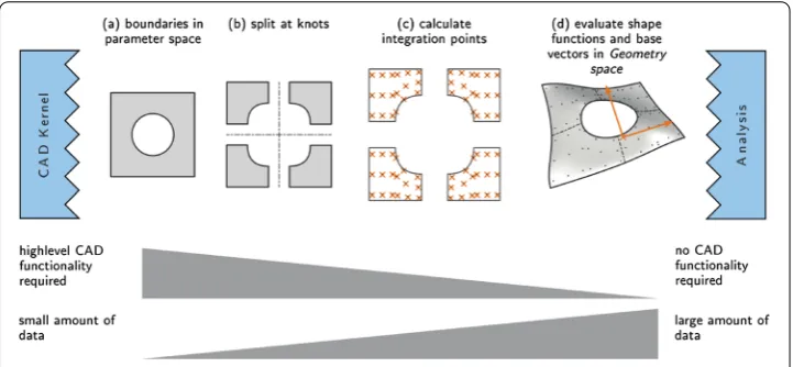
Fig. 9 Preparation of a trimmed surface for IBRA. Each step requires complex geometric functions. These functionalities can either be assigned to the CAD software or to the analysis tool. The complexity of the geometric requirements decrease to the right whereas the amount of data at the interface increases
Solver design
IBRA enables direct analysis of CAD-geometries. Figure9shows the preparation of the
CAD data for the finite element solver. A lot of complex geometric operations must be applied to provide the data for the solver. A complete IBRA solver environment would need only the basic geometrical data and do all these steps internally. The steps can also be done by uncoupled utility tools. This approach would create a large amount of data but allows conventional solvers to do IBRA without implementing additional functionality.
There are different ways to design an IBRA solver. Depending on the implemented func-tions the solver needs different kind of data. Using the example of the surface integration,
Fig.9shows different entry points for an analysis tool. In principle, the whole spectrum
of depicted interfaces between CAD and a solver is possible and in general it holds: A solver which is close to CAD needs a very high level of CAD functionalities and only a little amount of (complex) CAD data, whereas solvers without any dedicated build-in CAD functions require a big amount of rather basic data. Each step which reduces the CAD-related complexity of the solver (i.e. moving more “away” from CAD in direction of “classical FEM-solvers”), results in additional amount of data needed at the interface to the solver:
a. Read trimming data from CADboundary curves.
b. Split trimming domain at knotsboundary curves for each knot span.
c. Compute integration points for each spanset of integration points and weights. d. Evaluate all relevant data at the integration pointsbasis vectors, shape functions,
material properties, etc.
Thus, a complete IBRA analysis tool would only need the geometric CAD data in com-bination with the mechanical properties. It would be able to do the whole data processing
internally (Fig.9, leftmost).
This so calledmeshlessapproach allows to design a lightweight solver which only imple-ments the mechanical behaviour of the finite eleimple-ments but without any IBRA specific functionality.
In themeshlessenvironment each integration point contains the following data
• Shape function and derivativesthe evaluated values of the shape functions and deriva-tives respectively to each control point.
• Integration weightthe weighting factor for theGaussian quadrature.
• Control pointsthe locations and weights of the control points inGeometry space.
Storing the data for each integration point in an exchange file leads to large datasets. As a compromise, it is proposed within the present contribution to design an analysis tool with an interface for the integration points (after step c). In this way, the amount of data is reduced and the analysis tool needs only to provide some basic IGA functionalities for evaluating the geometry at the integration points.
Therefore, at least the following data must be available for each integration point
• Locationthe location of the quadrature point inParameter space. • Integration weightthe weighting factor for the Gaussian quadrature.
• Control pointsthe locations and weights of the control points inGeometry space. • Degreesthe degrees of the shape functions in each parameter direction.
• Knotsthe knot vectors in each parameter direction.
With this information the evaluation of the shape functions and the calculation of the base vectors can be performed (step d) using Eqs. (9) and (14).
Each integration point can carry additional information depending on the element type. Coupling elements for example require the tangents of the trimming curves within the
Parameter spaceof the underlying surface (see also Eq.11).
Note that the geometry refinement needs to be done in advance i.e. before creating the integration domains, since the solver is not capable to remesh the integration domain without the respective CAD functionalities. One loses the possibility of direct adaptive refinement if the given parametrization cannot resolve the structural behaviour.
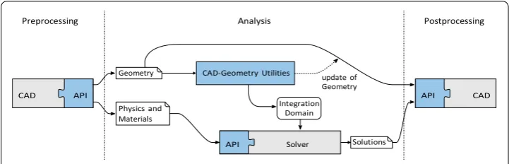
Design-through-analysis workflow
The goal of IBRA is to provide a general framework for bridging the gap between different CAD systems and FE solvers (see also [1]). Thus, in the following clear data interfaces are defined for an IBRA design-through-analysis workflow which allows such a seamless communication and a simulation directly based on the CAD data.
An overview of an IBRA design-through-analysis workflow is given in Fig.10. Note that
this is only exemplary for the proposed solver design in “Solver design” section. However, the workflow can be split and categorized into the following four software components
• CAD system for preprocessing.
• CAD-Geometry Utilities for determining the integration domains (trimmed surfaces
and B-Rep edges).
• FE solver for performing IBRA (with different CAD-related capabilities as described
in “Solver design” section).
Fig. 10 Exchange files and processes for an IBRA design-through-analysis workflow. The data inGeometry andIntegration domaincan be handled with the proposed IBRA exchange format. ThePhysics and Materials file is solver specific whereas theSolution datafile still requires an appropriate data format. The missing functionalities within CAD systems and FE solvers are added through correspondingapplication programming interfaces(APIs)
For the communication between these software components it turned out that the fol-lowing four data interfaces are useful
• Geometry.
• Integration domains.
• Physics and materials.
• Solutions.
This division into several interfaces provides modularity and allows that isogeometrically sophisticated as well as adapted standard FE-solvers find a docking point for processing the CAD-data. In the following, these data interfaces are explained briefly and specific exchange formats are developed and detailed in “IBRA exchange format” section.
Geometry
TheGeometrydata interface contains CAD data or more precisely NURBS-based B-Rep
models. It contains exclusively geometrical information whereas each entity has an id. These ids are used to assign analysis properties to the geometrical entities specified within
this file. The corresponding analysis data are specified within thePhysics and Materials
interfaces. TheGeometrydata can be written with an API in the desired CAD system. A
possible format of this interface is described in “Data interface—Geometry” section. Some
specific examples of theGeometrydata file are given in “Exchange format description for
geometry” section.
It can happen that during the preparation of theIntegration domainupdates in the CAD
geometries occur. This is the case for e.g. refinement operations. In this case theGeometry
data has to be updated. Thus, theCAD-Geometry Utilitieshas to provide functionalities
to updateGeometrydata (see Fig.10).
Physics and materials
The data interfacePhysics and Materials corresponds to the classical input file for an
FE solver just without geometry data. Using the ids employed within the data interface
Integration domains
Since the numerical integration of trimmed surfaces and along common edges is not a trivial task, it can be useful to outsource this task into a separate specialized library the
CAD-Geometry Utilities and to hand over just the required data for the IBRA element formulations. The required data for numerical integration of trimmed surfaces and edges
(see also Eqs. (9) and (14)) are defined in the data interface –Integration domainswhich
is described in “Data interface—Integration domains” section. The data can be exchanged within the applications in text files, for those the design is described in “Data interface— Integration domains” section. It can also be exchanged with more optimized interfaces
as e.g. data bases if theCAD-Geometry Utilitiesand the solver are strongly connected or
necessary interface connections are given.
The interface of theIntegration Domainscan be on different levels (see Fig.9). The IBRA
exchange format described in “Data interface—Integration domains” section refers to an exchange after computation of the integration points. It is advantageous if the interface happens between different software with interfaces that only allow import and export through text files. An exchange after the evaluation of shape functions and with it the base vectors became apparent to being more efficient for deeper integrated systems. All
geometry data is already precomputed by the CAD-Geometry Utilities. This strategy is
presented in “Data interface—Integration points” section.
Solutions
After computation, the solver writes the solution into files which can be used to visualize different results. The solution are either provided for the control points or for the inte-gration points in IBRA. In contrast to classical finite element analysis, IBRA uses also ids
for integration points. The IBRA solution data can be stored analogously to theGeometry
andIntegration domainfile. The only important thing is to use the same ID-systems in
order to have the results assignable to the initial files. In that case, theGeometryand
Inte-gration domaindata interfaces can be enriched by the solution data e.g. displacements or stresses from the FE solver. A visualization on the CAD model within a CAD system becomes possible. Alternatively, a visualization mesh can be created from the CAD model or integration points which allows also the visualization of IBRA results within an arbitrary postprocessing tool for classical FEA.
Exemplary implementations
The IBRA design-through-analysis workflow as presented in Fig.10has been implemented
for the finite element analysis packagesCarat++[55] andKRATOS-Multiphysiscs[56].
• Carat++ is a finite element software, developed at the author’s chair. It contains a complete set of CAD functionalities. Therefore it is possible to start an analysis
directly from theGeometryandPhysics and Materialsfiles.
• KRATOS-Multiphysiscs[56] is an open source finite element software started in 2001
by Dadvand, Rossi et al. [57,58]. An interface to theIntegration Domainallows to do
IBRA without the effort of implementing the necessary CAD functions.
• The plug-in TeDA has been developed for the CAD applicationsRhinoceros [59]
the assignment of mechanical properties to the geometric entities and the export of
GeometryandPhysics and Materialsfiles as well as ofIntegration Domainfiles.
IBRA exchange format
Within this paper, a format for the data interfaces GeometryandIntegration domains
is presented. As a format for the data, a JavaScript Object Notation (JSON) is used
because it is widely spread, flexible, easy to parse and a lot of libraries and useful tools are available for it. Even if an integrated data interface for the integration domains has big advantages e.g. performance or adaptive refinement, the proposed exchange format based on JSON is very useful in terms of the development of new B-Rep element for-mulations or the reduction of the implementation effort for using IBRA in a new FE solver to a minimum. Before describing the single components of the data interfaces
Geometry andIntegration domains, the ID system used within the exchange format is explained.
ID systems
Within the exchange format each entity requires an id, since geometry, integration domains and structural properties are separately stored. Hence, a unique link in between
has to be provided in order to allow also hybrids of the workflow shown in Fig.10. The
following id systems are used
• brep_id: This id is used to address the geometries of the topological entitiesbreps,
faces,edges, andvertices
• cp_id: This id is used to address the control points to which the degrees of freedom are enhanced.
• elem_idandquad_id: This id is used to address the integration domains (elements),
and quadrature points of the CAD model. Note that those ids are unique to thecp_id.
Thus, an element and node nor quadrature point cannot have the same id.
All ids are required for the data interfaceProject parameterwhich enhance the geometrical
entities with these ids by analysis data like boundary conditions or physical properties.
Data interface—Geometry
The data interfaceGeometrycontains all geometrical information of a NURBS-based
B-Rep model. It has to be as light as possible but still complete. Additionally it is desired that it is very easy to understand.
As changes can occur in the file design it gets aversion_number. The here proposed
design refers to number1.0.
Every CAD-model has some types oftolerance. It is important to know about the
toler-ances as the quality of the solution highly depends on it. Additionally during computation the knowledge about the tolerance is important to know about the correct convergence. As different CAD software uses distinct types of tolerances it is preferred to include a list of tolerances which can be specified by the chosen tools.
A surface B-Rep model consists of faces,edgesandvertices. The structure and
{
" v e r s i o n _ n u m b e r ": 1.0 , " t o l e r a n c e s ": [
l i s t o f t o l e r a n c e s ] ,
" b r e p s ": [ {
" b r e p _ i d ": i n t, " f a c e s ": [] , " e d g e s ": [] , " v e r t i c e s ": [ ] }
] }
Listing 1 Geometry – B-Rep
than one B-Rep. The structure of a B-Rep model is shown in Listing 1. The following
informations are necessary for each B-Rep:
• brep_id
• facessee Listing2 • edgessee Listing3 • verticessee Listing4.
Faces
A face is represented by a trimmed NURBS surface. An example of such a geometry is
shown in Fig.2.
An exemplary case of afacewithin the exchange format is given in Listing2. The format
consists of three main parts
• surfacedescribes the shape of the face i.e. the untrimmed NURBS surface. • boundary_loopsdescribes the boundaries of the surface.
• Theembedded_loops,embedded_curvesandembedded_pointsdefine embedded
entities which are used to address additional geometrical entities derived from the surface. They follow the same syntax as boundary entities (see below).
Additionally, the following information is needed
• brep_id
• swapped_surface_normalindicates if the surface normal of the surface needs to be swapped to have the correct orientation of the face.
The partsurfacedescribes the NURBS surface without B-Rep (trimming) information.
The following information are provided by
• is_trimmed:In the case the boundaries trim parts of the surface this flag is set TRUE. The flag is used for efficiency reasons.
• is_rational:In the case the flag is false all weights of the control points are equal to one. The flag is used for efficiency reasons.
• degrees:The polynomial degrees for the parametersuandv
• knot_vectors:The knot vectorsandHfor the parametersuandv
• control_pointsThe control points (CPs) have the idcp_id, their spatial position given as x-, y- and z-coordinates and their weights.
" f a c e s ": [{ " b r e p _ i d ": i n t,
" s w a p p e d _ s u r f a c e _ n o r m a l ": b o o l, " s u r f a c e ":
{
" i s _ t r i m m e d ": b o o l, " i s _ r a t i o n a l ": b o o l, " d e g r e e s ": [i n t,i n t] ,
" k n o t _ v e c t o r s ": [[d o u b l e, . . . ] , [d o u b l e, . . . ] ] , " c o n t r o l _ p o i n t s ": [
[d o u b l e c p _ i d ,
[d o u b l e p o s i t i o n _ x , d o u b l e p o s i t i o n _ y ,
d o u b l e p o s i t i o n _ z , d o u b l e w e i g h t ]] , . . . l i s t o f c o n t r o l p o i n t s
] } ,
" b o u n d a r y _ l o o p s ": [ {
" l o o p _ t y p e ": S t r i n g, O u t e r o r I n n e r " t r i m m i n g _ c u r v e s ": [
{
" t r i m _ i n d e x ": i n t, " c u r v e _ d i r e c t i o n ": b o o l, " p a r a m e t e r _ c u r v e ":{
" i s _ r a t i o n a l ": b o o l, " d e g r e e ": [i n t] ,
" k n o t _ v e c t o r ":[d o u b l e, . . . ] , " a c t i v e _ r a n g e ": [d o u b l e, d o u b l e] , " c o n t r o l _ p o i n t s ": [
[d o u b l e c p _ i d ,
[d o u b l e p o s i t i o n _ u , d o u b l e p o s i t i o n _ v , d o u b l e p o s i t i o n _ w , d o u b l e w e i g h t ] , ]
. . . l i s t of c o n t r o l p o i n t s ]
} } ,
. . . l i s t o f b o u n d a r y c u r v e s ]
} ,
. . . l i s t of b o u n d a r y l o o p s ] ,
" e m b e d d e d _ l o o p s ": [] , " e m b e d d e d _ c u r v e s ": [
{
" t r i m _ i n d e x ": i n t, " c u r v e _ d i r e c t i o n ": b o o l, " p a r a m e t e r _ c u r v e ":{
" i s _ r a t i o n a l ": b o o l, " d e g r e e ": [i n t] ,
" k n o t _ v e c t o r ": [d o u b l e, . . . ] , " a c t i v e _ r a n g e ": [d o u b l e, d o u b l e] , " c o n t r o l _ p o i n t s ": [
[d o u b l e c p _ i d ,
[d o u b l e p o s i t i o n _ u , d o u b l e p o s i t i o n _ v , d o u b l e p o s i t i o n _ w , d o u b l e w e i g h t ] ] ,
. . . l i s t o f c o n t r o l p o i n t s ]
} } ,
. . . l i s t of e m b e d d e d e d g e s ] ,
" e m b e d d e d _ p o i n t s ": [ {
" t r i m _ i n d e x ": i n t,
" p o i n t ": [d o u b l e p o s i t i o n _ u , d o u b l e p o s i t i o n _ v , d o u b l e p o s i t i o n _ w ] } ,
. . . l i s t of e m b e d d e d v e r t i c e s ]
} ,
. . . l i s t o f f a c e s ]
Listing 2 Geometry – Faces
• loop_type[Outer, Inner]: indicator specifies if loop is an outer or inner loop • trimming_curvescontains a set of respectively ordered curves (see also Fig.2).
The edges belonging to the corresponding face are listed intrimming_curves. Each edge
has
• trim_indexThis index is part of a local id system for each brep. • curve_directiondirection of the curve in the loop
• parameter_curvethe parameter curve describes the shape of the edge as a trimming curve in the parameter space of the corresponding face.
For theparameter_curvethe following information is provided
" e d g e s " : [ {
" b r e p _ i d ": i n t, " 3 d _ c u r v e ":
{
" d e g r e e ": [i n t] ,
" k n o t _ v e c t o r ": [d o u b l e, . . . ] , " a c t i v e _ r a n g e ": [d o u b l e, d o u b l e] , " c o n t r o l _ p o i n t s ":[
[d o u b l e c p _ i d ,
[d o u b l e p o s i t i o n _ x , d o u b l e p o s i t i o n _ y , d o u b l e p o s i t i o n _ z , d o u b l e w e i g h t ] ] ,
. . . l i s t o f c o n t r o l p o i n t s ]
} ,
" t r i m m m i n g _ r a n g e s ":[ {
" t r i m _ i n d e x ": i n t, " r a n g e ": [d o u b l e, d o u b l e] , } ,
. . . l i s t of t r i m m i n g r a n g e s ] ,
" t o p o l o g y ": [ {
" b r e p _ i d ": i n t, " t r i m _ i n d e x ": i n t, " r e l a t i v e _ d i r e c t i o n ": b o o l
} ] ,
" e m b e d d e d _ c u r v e s ": [] , " e m b e d d e d _ p o i n t s ": [] } ,
. . . l i s t o f e d g e s p o i n t s ]
Listing 3 Geometry – Edges
• knot_vectorsee above
• active_rangethe parameter curve is bounded by two vertices defined in the paramet-ric coordinate of the curve.
• control_pointsthe control points (CPs) have their spatial position given asu- and
v-coordinates and their weights in the parameter space of its face.
Points on the face can be described withinembedded_pointsas follows
• trim_indexsee above
• parameter_pointthe point is defined with the parametric coordinates of the surface
uandv.
Edges
A B-Rep edge is represented by a spatial NURBS curve (see also “Trimmed NURBS sur-faces” section). For an B-Rep edge the following information are provided
• brep_id
• 3d_curvecontains the information for describing the spatial curve representing the edge. Geometrical description given by degree, knot vector and control points. Addi-tionally, an active range is added for trimming.
• trimming_ranges
• topology describes the topology to the underlying geometrical information of the
edge (see also Fig.2)
• embedded_pointsandembedded_curvessee above.
Thetrimming_rangesare used for segmenting of the curve for e.g. coupling or boundary conditions and needs the following
" v e r t i c e s ": [ {
" b r e p _ i d ": i n t, " c o o r d i n a t e s ":
[d o u b l e c p _ i d ,
[d o u b l e p o s i t i o n _ x , d o u b l e p o s i t i o n _ y , d o u b l e p o s i t i o n _ z , d o u b l e w e i g h t ]] , " t o p o l o g y ": [
{
" b r e p _ i d ": i n t, " t r i m _ i n d e x ": i n t
}] } ,
. . . l i s t of v e r t i c e s ] ,
Listing 4 Geometry – Vertices
Thetopologyneeds the following
• brep_idrelated to the brep_id of its geometry
• trim_indexrelated to the trim_index of its trimming entity • relative_directiondirection of the edge to its trimming entity.
If notopologyis included, the here described description provides the definition of an
independent curve.
Vertices
A B-Rep vertex is represented by a spatial point. A vertex has the following information
• brep_id
• coordinatesx-, y-, and z-coordinates
• topology describes the topology to the underlying geometrical information of the vertex.
Note that only one assignment to either face or edge is necessary. Several assignments indicate a coupling.
Data interface—Integration domains
A novelty of the proposed exchange format is that it provides already the integration
domains for geometrical entities like faces andedges. Thus the implementation effort
on the FE solver side can be reduced to a minimum because the non-trivial numerical
integration of trimmed surfaces and common edges is outsourced Listing5.
The idea of the data structure is to provide for each quadrature point all necessary
infor-mation like location,weight, knot vectors etc. (see e.g. Eq.19). In addition, the integration
points are grouped to elements which in their turn are grouped to B-Rep entities, i.e. faces and edges. By having an id for each entity/group the correct assignment of analysis data can be guaranteed. The creation of these integration domains is performed by the library
as shown in Fig.10.
This work only explains the data structure for surfaces and its edges. The extension to curves and volumes can be derived straight forward.
The format consists of three main parts
• nodescontains all control points of the data interface specified in “Data interface— Geometry” section
{ " n o d e s ":[
[i n t c p _ i d ,
[d o u b l e p o s i t i o n _ x , d o u b l e p o s i t i o n _ y , d o u b l e p o s i t i o n _ z , d o u b l e w e i g h t ] ] ,
. . . l i s t o f n o d e s ] ,
" 2 d _ e l e m e n t s ": [ [i n t b r e p _ i d
[
[i n t e l e m e n t _ i d ,
[i n t d e g r e e _ u , i n t d e g r e e _ v ] , [ [d o u b l e k n o t _ v e c t o r , . . ] , [ . . , . . ] ] , [i n t c p _ i d , . . . ] ,
b o o l s w a p p e d _ n o r m a l , [
[i n t q u a d r a t u r e _ p o i n t _ i d ,
d o u b l e q u a d r a t u r e _ p o i n t _ w e i g h t i n g ,
[d o u b l e l o c a t i o n _ i n _ u , d o u b l e l o c a t i o n _ i n _ v ] , [ o p t i o n a l a d d i t i o n a l p r o p e r t i e s ]
] ,
. . . l i s t of q u a d r a t u r e _ p o i n t s ]
]
. . . l i s t of e l e m e n t s ] ,
. . . l i s t of p a t c h e s ] ,
" 1 d _ e l e m e n t s ": [] , " 3 d _ e l e m e n t s ": [] , " b r e p _ e l e m e n t s ":[ [i n t b r e p _ i d ,
[
[i n t b r e p _ e l e m e n t _ i d , [
[i n t e l e m e n t _ i d , o p t i o n a l e l e m e n t _ i d o f s l a v e e l e m e n t s] , [ [i n t q u a d r a t u r e _ p o i n t _ i d ,
d o u b l e w e i g h t i n g ,
[d o u b l e l o c a t i o n _ i n _ u , d o u b l e l o c a t i o n _ i n _ v ] , [d o u b l e t a n g e n t _ t _ x i , d o u b l e t a n g e n t _ t _ e t a ] , [ o p t i o n a l p r o p e r t i e s r e l a t e d t o d e g r e e s o f f r e e d o m ] , [ o p t i o n a l l o c a t i o n in s l a v e e l e m e n t ] ,
[ o p t i o n a l t a n g e n t s of s l a v e e l e m e n t t r i m ] ]
]
. . . l i s t of q u a d r a t u r e p o i n t s ]
] ,
. . . l i s t of b r e p _ e l e m e n t s ] ,
. . . l i s t o f b r e p s ]
] }
Listing 5 Element Formulation
Nodes
The set of nodes is optional because the control points are already listed within the data
interface “Data interface—Geometry” section (see faces). Nevertheless for a faster and
easier parsing it can make sense to duplicate them in a separate list.
Elements
The proposed exchange format allows 1D, 2D, and 3D geometries whereas the dimension
refers to the dimension of theParameter space:
• 1d_elements: curved structures, possible element types are e.g. beams or trusses. • 2d_elements: surfaces, possible element types are e.g. plates, membranes or shells. • 3d_elements: solids.
This section explains exemplarily the components of the2d_elements. The elements
are grouped to B-Rep entities having a corresponding brep_id(see also data interface
Geometry). Each element has the following information:
• element_id
• degrees