High order cut finite element methods
for the Stokes problem
August Johansson
1*, Mats G. Larson
2and Anders Logg
3Background Introduction
Meshing of complex geometries remains a challenging and time consuming task in engi-neering applications of the finite element method. There is therefore a demand for finite element methods based on more flexible mesh constructions. One such flexible mesh paradigm is the formulation of finite element methods on composite meshes created by letting several meshes overlap each other. This approach enables using combinations of meshes for certain parts of a domain and reuse of meshes for complicated parts that may have been difficult and time consuming to construct.
We consider the case of a composite mesh consisting of one mesh that overlaps another mesh which together provide a mesh of the computational domain of interest. This results in some elements on one mesh having an intersection with one or several elements on the boundary of the other mesh. We denote such elements by cut elements. The interface conditions on these cut elements are enforced weakly and consistently using Nitsche’s method [1].
In this setting [2] first developed and analyzed a composite mesh method for elliptic second order problem based on Nitsche’s method. In [3], this approach was extended to the Stokes problem using suitable stabilization to ensure inf-sup stability of the method. Implementation aspects were discussed in detail in [4]. In [5] a related cut finite element method for a Stokes interface problem based on the P1-iso-P2 element was developed and analyzed.
Abstract
We develop a high order cut finite element method for the Stokes problem based on general inf-sup stable finite element spaces. We focus in particular on compos-ite meshes consisting of one mesh that overlaps another. The method is based on a Nitsche formulation of the interface condition together with a stabilization term. Starting from inf-sup stable spaces on the two meshes, we prove that the resulting composite method is indeed inf-sup stable and as a consequence optimal a priori error estimates hold.
Keywords: Interface problem, High order, Stokes problem, Nitsche’s method, Unfitted finite element methods
Open Access
© 2015 Johansson et al. This article is distributed under the terms of the Creative Commons Attribution 4.0 International License (http://creativecommons.org/licenses/by/4.0/), which permits unrestricted use, distribution, and reproduction in any medium, provided you give appropriate credit to the original author(s) and the source, provide a link to the Creative Commons license, and indicate if changes were made.
RESEARCH ARTICLE
Composite mesh techniques using domain decomposition are often called chimera, see for example [6, 7] for uses in a finite difference setting or [8] in a finite element set-ting. The extended finite element method (XFEM) also provides composite mesh han-dling techniques, see for example [9, 10]. However, the Nitsche method approach using cut elements used in this work makes it possible to obtain a consistent and stable formu-lation while maintaining the conditioning of the algebraic system for both conforming and non-conforming high order finite elements.
In this paper, we consider Stokes flow and devise a method based on a stabilized Nitsche formulation for enforcement of the interface conditions at the border between the two meshes. A specific feature is that we only assume that we have inf-sup stable spaces on the two meshes and that the spaces consist of polynomials. We can then show that our stabilized Nitsche formulation satisfies an inf-sup condition and as a conse-quence optimal order a priori error estimates hold. We emphasize that the spaces are arbitrary and can be different on the two meshes, in particular, continuous or discontin-uous pressure spaces as well as higher order spaces can be used. We present numerical results for higher order Taylor-Hood elements in two and three spatial dimensions that confirm our theoretical results.
The outline of the paper is as follows: First we review the Stokes problem. Then the finite element method is presented by first defining the composite mesh and introducing finite element spaces. The method is then analyzed where the inf-sup condition is the main result. Finally we present the numerical results and the conclusions.
The Stokes problem
In this section, we review the Stokes problem and state its standard weak formulation. We also introduce some basic notation.
Strong form
Let be a polygonal domain in Rd with boundary ∂�. The Stokes problem takes the form: Find the velocity u:→Rd and pressure p:→R such that
where f :→Rd is a given right-hand side. Weak form
As usual, let Hs(�) denote the standard Sobolev space of order s≥0 on with norm denoted by � · �Hs(�) and semi-norm denoted by | · |Hs(�). Let L2(�) denote the L2-norm on with norm denoted by � · �. The corresponding inner products are labeled
accord-ingly. We will also use the notation xy to denote the inequality x≤Cy, where C is a
constant. The corresponding inequality xy is defined accordingly. Introducing the spaces
(1) −u+ ∇p=f in,
(2) divu=0 in,
(3) u=0 on∂�,
with norms �Dv�= �v⊗ ∇� and q, the weak form of (1) and (2) reads: Find (u,p)∈V ×Q such that
where the forms are defined by
Remark 1 We obtain the variational problem (6) by formally multiplying (1) by a test function v and (2) by a test function −q.
It is then possible to show that the inf-sup condition
holds, from which it follows that there exists a unique solution to (6). See [11] for further details.
Method
The composite mesh
We here present the concepts and notation of the domains and meshes used. The main idea is to introduce a background domain which is partially overlapped by another domain (the overlapping domain). For each of these domains, we mimic the setup of a traditional finite element method in the sense that each domain is equipped with a tra-ditional finite element mesh. The two meshes are completely unrelated. In particular, the interface between the two meshes is determined by the overlapping domain and is not required to match or align with the triangulation of the background domain.
The composite domain
Let the predomainsi ⊂, i=0, 1, be polygonal subdomains of in Rd such that
0∪1=; see Fig. 1. Consider the partition
and let Ŵ=∂�1\∂� be the interface between the overlapping domain 1 and the under-lying domain 0; see Fig. 1. We make the basic assumption that each i, i=0, 1, has a nonempty interior. We note that implies that there exists a nonempty open set U ∈ such that Ŵ∩U �= ∅ (The set U plays an important role in the proof of Lemma 4 below).
(5)
Q= {q∈L2(�):
�
qdx=0},
(6) a(u,v)+b(u,q)+b(p,v)=l(v) ∀(v,q)∈V×Q,
(7) a(u,v)=(Du,Dv)�,
(8) b(u,q)= −(divu,q)�
(9) l(v)=(f,v)�.
(10)
�q��sup
v∈V
b(v,q)
�Dv��
=sup v∈V
(divv,q)
�Dv��
∀q∈Q
The composite mesh
For i=0, 1, let Kh,i be a quasi-uniform mesh on i with mesh parameter h∈(0,h]¯ and let
be the submesh consisting of elements that intersect i; see Fig. 2. Note that Kh,0 includes elements that partially intersect 1. We also introduce the notation
Note that 1=h,1 and 0⊂h,0; see Fig. 3.
We obtain a partition of by intersecting the elements with the subdomains:
See also Fig. 2.
(12) Kh,i= {K ∈Kh,i:K∩i�= ∅}
(13) h,i =
K∈Kh,i K.
(14) 1
i=0
Kh,i∩i= 1
i=0
{K∩i:K ∈Kh,i}.
Ω
0Ω
1Ω
0Ω
1=
Ω
1Γ
Fig. 1 The domains i and the subdomains i (all shaded) sharing the interface Ŵ
K
h,0K
h,1K
h,0K
h,1=
K
h,1Γ
Fig. 2 The meshes Kh,i and Kh,i of the corresponding domains i and h ,i. Note that Ŵ is not aligned with Kh,0
Ω
h,
0
Ω
h,
1
= Ω
1
Γ
Finite element formulation
In this section, we present the finite element method for approximating the weak form (6). Some notation will be introduced, but the main idea is to assume we have inf-sup stable spaces in each of the subdomains away from the interface. Then we are able to for-mulate a method similar to [2] and [3].
Finite element spaces
For each of the predomains i with corresponding family of meshes Kh,i we consider velocity and pressure finite element spaces Vh,i×Qh,i. The spaces do not contain bound-ary or interface conditions since these will be enforced by the finite element formulation. We define
where i=0, 1 and define
Note that since the domains h,i overlap each other, Vh×Qh is to be understood as a collection of function spaces on the overlapping patches h,i, i=0, 1. Using the notation
Y(x) to denote the average of x over the domain Y, we now make the following funda-mental assumptions on these spaces:
Assumption A (Piecewise polynomial spaces) The finite element spaces Vh and Qh con-sist of piecewise polynomials of uniformly bounded degree k and l, respectively.
Assumption B (Inf-sup stability) The finite element spaces are inf-sup stable restricted to a domain bounded away from the interface. More precisely, we assume that for i=0, 1 and h∈(0,h]¯ there is a domain ωh,i⊂�i such that:
(a) The set ωh,i is a union of elements in Kh,i; see Fig. 4.
(b) The inf-sup condition
(15) Vh,i×Qh,i=Vh,i|h,i×Qh,i|h,i,
(16) Vh×Qh=
1
i=0
Vh,i×Qh,i.
(17)
mi�pi−ωh,i(p)�ωh,i≤ sup
v∈Wh,i
(divv,p)ωh,i
�Dv�ωh,i
ω
h,0
ω
h,1
= Ω
h,1
Γ
holds, where Wh,i is the subspace of Vh,i defined by
(c) The set ωh,0 is close to 0 in the sense that
where Uδ(Ŵ)= {x∈Rd: |ρ(x)|< δ} is the tubular neighborhood of Ŵ with thick-ness δ.
Remark 2 The assumptions presented ensure that the polynomial spaces are such that certain inverse inequalities hold. More generally, inverse inequalities hold if there is a finite set of finite dimensional reference spaces used to construct the element spaces. The use of the interpolant in the proof of Lemma 4 could alternatively be handled using an abstract approximation property assumption.
Finite element method
We consider the finite element method: Find (uh,ph)∈Vh×Qh such that
where the forms are defined by
Here, n is the unit normal to Ŵ exterior to 1. Denoting the restriction of v to i by vi =v|i, [v] =v1−v0 is called the jump and �v� =(v0+v1)/2 is called the
aver-age. (Any convex combination for the average is valid [2].) The parameter β >0 is the Nitsche parameter and must be sufficiently large (see for example [2]) and scales as k2, (18)
Wh,0= {v∈Vh,0:v=0 on�h,0\ωh,0},
(19)
Wh,1=Vh,1.
(20) �h,0\ωh,0⊂Uδ(Ŵ), δ∼h,
(21) Ah((uh,ph),(v,q))=lh(v) ∀(v,q)∈Vh×Qh,
(22) Ah((u,p),(v,q))=ah(u,v)+bh(u,q)+bh(v,p)+dh((u,p),(v,q)),
(23) ah(u,v)=ah,N(u,v)+ah,O(u,v),
(24)
ah,N(u,v)=(Du,Dv)�0+(Du,Dv)�1
−(�(Du)·n�,[v])Ŵ−([u],�(Dv)·n�)Ŵ
+βh−1([u],[v])Ŵ,
(25) ah,O(u,v)=([Du],[Dv])�h,0∩�1,
(26)
bh(u,q)= −(divu,q)�0−(divu,q)�1+([n·u],�q�)Ŵ,
(27) dh((u,p),(v,q))=h2(�u− ∇p,�v+ ∇q)�h,0\ωh,0,
where k is the polynomial degree. Furthermore, h is the representative mesh size of the quasi-uniform mesh. In a practical implementation, h is evaluated as the local element size.
A comment on the respective terms may be clarifying:
• ah,N (and the last term in bh) contains the standard Nitsche formulation of (6) to
enforce continuity over the interface. This is similar to an interior penalty discontinu-ous Galerkin method [12].
• ah,O is a stabilization of the jump of the gradients across Ŵ (see [3]). This term is
to avoid ill-conditioning when the intersection of an element and the domain is small.
• dh (and the last term in lh) stabilizes the method since we do not assume inf-sup
sta-bility in all of 0. This least-squares type of stabilization is commonly found in low-order methods, see e.g. [13] for more details.
By simple inspection, we note that the method is consistent. We conclude by noting that the method satisfies the Galerkin orthogonality.
Proposition 1 (Galerkin orthogonality) Let (u,p)∈V×Qbe a weak solution to the
formulation (6) and let(uh,ph)∈Vh×Qh be the solution to the finite element formula-tion (21). Then it holds
Proof The result follows from [2] and noting that ah,O(u,vh)=dh((u,p),(vh,qh))=0
for all (vh,qh)∈Vh×Qh.
Approximation properties
We assume that there is an interpolation operator πh,i:Vi(�h,i)→Vh,i, for i=0, 1,
where Vi(�h,i)⊂ [L2(�h,i)]d is a space of sufficient regularity to define the interpolant.
For Taylor-Hood elements, we take πh,i to be the Scott-Zhang interpolation
opera-tor [14], and Vi(�h,i)= [L2(�h,i)]d. For other elements we refer to their corresponding papers, for example the Crouzeix-Raviart element [15], the Mini element [16], or the overviews in [13] or [17].
The full interpolation operator πh:V→Vh can now be defined by the use of a linear
extension operator E: [Hs(ωh,0)]d → [Hs(�h,0)]d, s≥0, such that (Ev)|ωh,0 =v and
Now, πh:V→Vh is defined by
A similar argument can be made to define the pressure interpolation operator πh:Q→Qh.
Furthermore, we assume that the following standard interpolation estimate holds: (29) Ah((u,p)−(uh,ph),(vh,qh))=0 ∀(vh,qh)∈Vh×Qh.
(30) EvHs(�
h,0)vHs(ωh,0).
(31)
πhv=πh,0Ev0⊕πh,1v1.
(32)
�v−πhv�Hm(K)hk+1−m|v|
Here, in the case of a Scott-Zhang interpolation operator, K is the patch of elements
sharing a vertex with element K.
Stability and convergence
In this section, we prove that the finite element method proposed in (21) is stable. This is done by first proving the coercivity and continuity of ah defined in (23), followed by
proving that bh defined in (26) satisfies the inf-sup condition. Combining these results
proves stability of Ah. This strategy is similar to what can be found in [3] and [5]. In
particular, Verfürth’s trick [18] is used to prove inf-sup stability. For a general overview of the saddle point theory used, see [11, 13, 17]. We conclude the section by proving an a priori error estimate. Before we begin, we state appropriate norms.
Norms
In the analysis that follows, we shall use the following norms:
Interpolation estimates
Using (32) together with the trace inequality �v�2Ŵ∩K h−1�v�2K +h�∇v�2K, we obtain
the following interpolation estimate for v∈V:
See [2] for a proof. For the pressure p, we have
Coercivity and continuity
Establishing coercivity and continuity of ah is straightforward and similar to [2].
Lemma 1 (Coercivity of ah) The bilinear formah (23) is coercive:
Proof Note that the overlap term ah,O provides the control
(33)
|||v|||2h=
1
i=0
�Dvi�2�h,i+h��Dv� ·n�
2 Ŵ+h
−1�[
v]�2Ŵ, v∈Vh,
(34) �q�2h=
1
i=0
�qi�2h,i, q∈Qh,
(35)
|||(v,q)|||2h= |||v|||2h+ �q�2h, (v,q)∈Vh×Qh.
(36) |||v−πhv|||hhk|v|
Hk+1(�).
(37) �p−πhp�hhl+1|v|Hl+1(�).
where we have used that h,0\1=0 and h,0∩1⊂1 as described in the section on the composite mesh above. We also note that for each element K that intersects an interface segment Ŵ we have the inverse bound
independent of the particular position of the intersection between K and Ŵ (see [2]).
Combining these two estimates with the standard approach to establish coercivity of a Nitsche method (see for example [2]) immediately gives the desired estimate.
Lemma 2 (Continuity of ah) The bilinear formah (23) is continuous:
Proof A proof in absence of ah,O is found in [2]. Bounding ah,O is straightforward using
the Cauchy-Schwarz inequality and the fact that �Dw�h,i|||w|||h for any w∈Vh and
i=0, 1.
Stability
Showing stability of the proposed finite element method involves several steps. First we show a preliminary stability estimate for Ah (21). Then the so called small inf-sup
condi-tion for bh (26) is shown using a decomposition of the pressure space into L2 orthogonal
components. For each of these components we show that an inf-sup condition holds. This is then used to show the big inf-sup condition for Ah.
Lemma 3 (Preliminary stability estimate for Ah) It holds
Proof Recall the inverse estimate
(see [19], Section 4.5) where m,l∈Z+, K ∈Kh,i and v∈Vh. The first estimate in the lemma follows by adding and subtracting u, using the triangle inequality and (43) as follows:
(39) 1
i=0 �Dv�2�
h,i= �Dv0� 2
�h,0\�1+ �Dv0� 2
�h,0∩�1+ �Dv1� 2 �h,1
�Dv0�2�
h,0\�1+ �D(v0−v1)� 2
�h,0∩�1+ �Dv1� 2 �1
≤ 1
i=0
�Dv�2�i+ah,O(v,v),
(40) h�(Dv)·n�2K∩Ŵ �Dv�2K
(41) ah(v,w)|||v|||h|||w|||h ∀v,w∈Vh.
(42) |||u|||2h+h2�∇p�2�
h,0\ωh,0 |||u|||
2
h+h
2
��u− ∇p�2�
h,0\ωh,0
Ah((u,p),(u,−p)).
(43) �v�Hl(K)≤Chm−l�v�Hm(K)
(44) h2�∇p�2K ≤h2�∇p−u�2K +h2�u�2K
for each element K ∈Kh,i. The second estimate follows immediately using coercivity (38) since
The pressure space can be written as the following L2-orthogonal decomposition:
where Qc is the space of piecewise constant functions on the partition {i}1i=0 of with
average zero over and Qi is the space of L2 functions with average zero over i. We next show inf-sup conditions for Qc and Q0. Recall that the inf-sup condition for Q1 is already established by Assumption B.
Lemma 4 (Inf-sup for Qc) For eachq∈Qcthere exists awc∈Vh with|||wc|||h= �q�h such that
where the bound is uniform w.r.t. q.
Proof We first note that Qc is a one-dimensional vector space spanned by
and that we have the identities
Second, we note that since 0 and 1 are nonempty, there exists a nonempty open set
U ⊂ such that Ŵ∩U �= ∅. Let now x0∈Ŵ∩U be a point on the interface Ŵ and let BR(x0) be a ball of radius R centered at x0 as in Fig. 5. The radius R is chosen such that
BR(x0)⊂U independently of the mesh size h.
Now, let γ =Ŵ∩BR(x0) and note that on γ, both the interface normal n and the jump
[χ] are constant [In fact, [χ] is constant on the entire interface, see (49)].
To construct the test function wc∈Qc, we let ϕ be a smooth nonnegative function
compactly supported on BR(x0) such that ϕ=1 on BR/2(x0), and take v(x)=cϕ(x)n,
where c is a constant to be chosen. We then have the identity
Choosing c= |γ|−1 we obtain
Integrating by parts and recalling that χ is constant on each subdomain i, i=0, 1, it fol-lows that this construction of v leads to the identity
(45) Ah((u,p),(u,−p))=ah(u,u)+dh((u,p),(u,−p))
=ah(u,u)+h2�∇p−�u�2�h,0\ωh,0
|||u|||2h+h2�∇p−�u�2�
h,0\ωh,0.
(46)
Q=Qc⊕Q0⊕Q1,
(47) q2hbh(wc,q),
(48)
χ=
|�0|−1 in�0,
−|�1|−1 in�1.
(49)
�χ�2�= |�1|−1+ |�2|−1, [χ] = −|�1|−1+ |�2|−1= −�χ�2�
(50)
(�n·v�,[χ])γ =(�n·cϕn�,[χ])γ = −c|γ| �χ�2�.
Now, let w=πhv∈Vh. It follows that
The last inequality holds for all h∈(0,h]¯ with h¯ sufficiently small. (Note that the con-stants c and C do not depend on q). The first inequality follows by noting that
Here we have first used the Cauchy-Schwarz inequality, then a trace inequality on BR(x0) and the second identity of (49) to replace |[χ]| by χ� , then an inequality of
the type aba2+b2 and the interpolation estimate (32), and finally the estimate ϕH2(BR(x0))1, which holds since ϕ is a fixed compactly supported smooth function.
Finally, given q∈Qc, we may write q=c1χ for some c1>0. (If c1<0, we may rede-fine χ). Taking wc=c2w, where c2>0 is chosen such that |||wc|||h= �q�h, we have
where we used the fact that χhχ�, which holds since χ is piecewise constant and
|�h,0\�0|h|Ŵ|1, and the identities c1= �q�h/�χ�� and c2= �q�h/|||w|||h to
con-clude that c1/c2= |||w|||h/�χ��∼1, since w and χ are both fixed functions.
(52)
bh(v,χ )= −(�n·v�,[χ])γ = �χ�2�.
(53) bh(w,χ )=bh(v,χ )+bh(w−v,χ )
= �χ�2�−(�n·(w−v)�,[χ])γ
= �χ�2�−c(�πhϕ−ϕ�,[χ])γ
≥ �χ�2�−cCh�χ�2�
�χ�2�.
(54)
|(�πhϕ−ϕ�,[χ])γ| ≤ ��πhϕ−ϕ��γ�[χ]�γ
= ��πhϕ−ϕ��γ|γ|1/2|[χ]|
�πhϕ−ϕ�1BR(/2x0)�πhϕ−ϕ�1H/12(BR(x 0))�χ�
2
�
h�∇ϕ�BR(x0)+ ��ϕ�BR(x0)
�χ�2�
h�χ�2�.
(55) bh(wc,q)=c1c2bh(w,χ )
c1c2�χ�2�
c1c2�χ�2h
= c2 c1
�q�2h
�q�2h,
x
0
B
R
(x
0
)
Γ
Remark 3 We may generalize the proof to a more general assumption on the inter-face between the overlapping domain 1 and underlying domain 0 as follows. Con-sider the situation where the interface Ŵ is piecewise smooth and for each value of the
mesh parameter h, 1,h is a polygonal domain consisting of shape regular tetrahedra that approximates 1 in such a way that the resulting surface mesh on ∂�1,h interpolates ∂�1. Then for each value of h we obtain a piecewise linear interface Ŵh, with unit normal nh,
approximating the piecewise smooth interface Ŵ.
Let x0∈Ŵ and assume that x0 and R are chosen such that γ =BR(x0)∩Ŵ is smooth. We define v(x)=cϕ(x)n(x0) and, instead of (51), we obtain
where γh=BR(x0)∩Ŵ. With our assumptions we find that for R and h¯ small enough, there are constants c1,c2>0 such that
In fact |γh| → |γ| as h→0, and if we for each x∈γh let p(x) be the closest point on Ŵ we
have
where the first term tends to zero as h tends to zero and the second is positive for a suffi-ciently small R, since the curvature is bounded and therefore the normal varies continu-ously with the distance from x0. Choosing the constant c=1/(c1c2) in (56), we obtain
The proof may now be continued in the same fashion as for fixed polygonal domains.
Lemma 5 (Inf-sup for Q0) For each q∈Q0 there exists a w∈Wh,0⊂Vh,0 with �Dw�ωh,0 = �q−ωh,0(q)�ωh,0 such that
where the bound is uniform w.r.t. q.
Proof Recall the definitions of Wh,0 and ωh,0 from Assumption B. We first show that we can change the average from �0(q) to ω
h,0(q) using the following estimates:
where we first added and subtracted ω
h,0(q) and used the triangle inequality, then used the identity ωh,0(q)=�0(ωh,0(q)), which holds since 0 is an average, and finally we used the L2(�h,0) stability |�
0(v)|�v��h,0 of the average operator.
(56) (�nh·v�,[χ])γh= −c|γh|nh·n(x0)�χ�
2
�
(57) |γh| ≥c1, nh(x)·n(x0)≥c2 ∀x∈γh, ∀h∈(0,h0]
(58) nh(x)·n(x0)=(nh(x)−n(p(x)))·n(x0)+n(p(x))·n(x0)
(59)
−(�nh·v�,[χ])γ =c|γh|nh·n(x0)�χ�2�≥cc1c2�χ�2�≥ �χ�2�
(60) �q−�0(q)�2
�h,0 −h 2�∇
q�2�
h,0\ωh,0 bh(w,q),
(61)
�q−�
0(q)��h,0 ≤ �q−ωh,0(q)��h,0+ �ωh,0(q)−�0(q)��h,0 = �q−ω
h,0(q)��h,0+ ��0(ωh,0(q)−q)��h,0
�q−ω
Next we have the estimate
which follows by first observing that this inverse inequality holds:
where K1 and K2 are two neighboring elements sharing the face F12. Then, starting with
ω0h,0=ωh,0, we define a sequence of sets ωhn,0, n=1, 2,. . . consisting of the union of ωnh,0−1 and all elements K⊂�h,0\ωhn−,01 that share a face with an element in ωnh−1,0 . It then
fol-lows from (64) that
Using the assumption that ωh,0 is close to 0 (20) together with shape regularity and quasi-uniformity of the mesh we conclude that ωhn,0=�h,0 for some n≤C for all h∈(0,h]¯ where the constant is independent of h. Now (62) follows from a uniformly bounded number of iterations of (65).
Combining (61) with (62), we obtain
where we used the fact that ∇ωh,0(q)=0 and at last the inf-sup condition (17) to choose a w0∈Wh,0 with �Dw0�ωh,0 = �q−ωh,0(q)�ωh,0 such that bh(w0,q)= �q−ωh,0(q)�
2
ωh,0.
We now combine the inf-sup estimates for Qc and Q0 to prove an inf-sup estimate for Qh.
Lemma 6 (Small inf-sup) There are constants C>0 andm>0 such that for each
q∈Qh there exists aw∈Vh with|||w|||h= �q�h such that
where the bound is uniform w.r.t. q.
Proof Take wc as in Lemma 4, w0 as in Lemma 5 and w1∈Wh,1. Consider the test function w=δ1wc+w0+w1 where δ1>0 is a parameter. By writing
q=qc+q0+q1∈Qc⊕Q0⊕Q1, we have
(62)
�q�2�
h,0 �q�
2
ωh,0+h
2�∇
q�2�
h,0\ωh,0 ∀q∈Q0,
(63)
�q�2K 1 h
2�∇ q�2K
1+h�q�
2 F12
(64)
�q�2K1 h2�∇q�2K1+ �q�2K2,
(65) �q�2ωn
h,0 �q�
2
ωnh,0−1+h
2�∇ q�2
ωnh,0\ωnh,0−1, n=1, 2,. . .
(66) �q−�
h,0(q)� 2
�h,0 �q−ωh,0(q)� 2 �h,0
�q−ω
h,0(q)� 2 ωh,0+h
2
�∇q�2�h,0\ωh,0
bh(w0,q)+h2�∇q�2�h,0\ωh,0,
(67)
m�q�2h−Ch2�∇q0�2�
Note that bh(wi,qc)=0, i=0, 1. This follows from integration by parts since qc∈Qc, which is piecewise constant, and since wi∈Wh,i, which is zero on the boundary. The
second term and third terms on the right-hand side can be estimated as follows
where i=0, 1 and δ2>0 is a parameter. Here we have used the bound �divv� ≤ �Dv�, the definition of wc from Lemma 4 and Young’s inequality
ab≤ǫa2+(4ǫ)−1b2≤ǫa2+ǫ−1b2, which holds for any ǫ >0. Continuing from (68), we use (69) to obtain
where we first choose δ2 sufficiently small and then δ1 sufficiently small to ensure that the
two first terms are positive.
Finally, we note that by construction
and thus |||w|||h�q�h. The desired result now follows by setting w = �q�h(w/|||w|||h), which gives
(68) bh(δ1wc+w0+w1,q)=δ1bh(wc,qc)+δ1bh(wc,q0)+δ1bh(wc,q1)
+bh(w0,qc)
=0
+bh(w0,q0)+bh(w0,q1)
=0 +bh(w1,qc)
=0
+bh(w1,q0)
=0
+bh(w1,q1)
≥δ1mc�qc�2h−δ1|bh(wc,q0)| −δ1|bh(wc,q1)|
+m0�q0−� 0(q0)�
2
�h,0−Ch
2�∇q0�2
�h,0\ωh,0
+m1�q1−� 1(q1)�
2
�1 =⋆.
(69) δ1|bh(wc,qi)| =δ1|bh(wc,qi−�h,i(qi))|
δ1�Dwc��h,i�qi−�h,i(qi)��h,i δ1�qc��h,i�qi−�i(qi)��h,i
δ12δ2−1�qc�h2+δ2�qi−�i(qi)� 2
�h,i,
(70) ⋆≥δ1
mc−Cδ1δ2−1
�qc�2h+
1
i=0
(mi−Cδ2)�qi−�h,i(qi)�
2
�h,i
−Ch2�∇q0�2�h,0\ωh,0
�m
�qc�2h+
1
i=0
�qi−� i(q)�
2
�h,i
= �q�h
−h2�∇q0�2�h,0\ωh,0,
(71)
|||w|||2h|||wc|||2h+
1
i=0
|||wi|||2h
= �qc�2h+
1
i=0
�qi�2h,i
Proposition 2 (Big inf-sup) It holds
Proof Given p∈Qh, take w∈Vh as in Lemma 6. First note that for dh we have the
estimate
where we have used the Cauchy-Schwarz inequality, the triangle inequality, the inverse estimate (43), the definition of the energy norm (33) and the definition of w in Lemma 6.
Next for δ1>0 we have
where we have used Lemmas 3, 2, 6 as well as (74). Choosing first δ2 sufficiently small
and then δ1 sufficiently small, we arrive at the estimate
We now note that
(72)
bh(w,q)= �q�h
|||w|||hbh(w,q)
bh(w,q).
(73)
|||(u,p)|||h sup
(v,q)∈Vh×Qh
Ah((u,p),(v,q))
|||(v,q)|||h .
(74) |dh((u,p),(w, 0))|h2��u− ∇p��h,0\ωh,0��w��h,0\ωh,0
h2��u��h,0\ωh,0 + �∇p��h,0\ωh,0
��w��h,0\ωh,0
�Du��h,0\ωh,0+h�∇p��h,0\ωh,0
�Dw��h,0\ωh,0
δ2−1
�Du�2�
h,0\ωh,0+h 2�∇p�2
�h,0\ωh,0
+δ2�Dw�2�h,0\ωh,0
δ2−1
|||u|||2h+h2�∇p�2� h,0\ωh,0
+δ2�p�2h,
(75) Ah((u,p),(u,−p)+δ1(w, 0))=Ah((u,p),(u,−p))
+δ1
ah(u,w)+bh(w,p)+dh((u,p),(w, 0))
|||u|||2h+h2�∇p�2�h,0\ωh,0
−δ1
δ2−1|||u|||2h+δ2�p�2h
+δ1
�p�2h−h2�∇p�2�h,0\ωh,0
−δ1δ2−1
|||u|||2h+h2�∇p�2�h,0\ωh,0
−δ1δ2�p�2h
1−Cδ1δ−21
|||u|||2h+
1−Cδ1δ2−1
h2�∇p�2�
h,0\ωh,0
+δ1(1−Cδ2)�p�2h,
(76)
|||(u,p)|||2h= |||u|||2h+ �p�2h
and thus the desired estimate (73) follows since
A priori error estimate
In this section we use the approximation properties of the finite element spaces to show that the proposed method is optimal.
Theorem 1 It holds
Proof By the triangle inequality we have
From the approximation property (36), we obtain an optimal estimate of the first term. To show an optimal estimate for the second term we recall the big inf-sup estimate Proposition 2
where we have used a pair (vh,qh) such that |||(vh,qh)|||h1 in the inequality and the Galerkin orthogonality (29) to obtain the equality. The terms in Ah (22) may now be
esti-mated individually. The optimal estimate for ah (23) follows immediately from continuity (41). For bh(u−πhu,qh) (26) we have
(77)
|||(u+δ1w,−p)|||2h= |||u+δ1w|||2h+ �p�2h
≤ |||u|||2h+δ1|||w|||2h+ �p�2h
|||u|||2h+ �p�2h
= |||(u,p)|||2h.
(78)
|||(u,p)|||h
Ah((u,p),(u+δ1w,−p))
|||(u,p)|||h
Ah((u,p),(u+δ1w,−p))
|||(u+δ1w,−p)|||h
.
(79)
|||(u,p)−(uh,ph)|||hhk(�u�Hk+1(�)+ �p�Hk(�)).
(80) |||(u,p)−(uh,ph)|||h|||(u,p)−(πhu,πhp)|||h+ |||(πhu,πhp)−(uh,ph)|||h.
(81)
|||(πhu,πhp)−(uh,ph)|||hAh((πhu,πhp)−(uh,ph),(vh,qh))
=Ah((πhu,πhp)−(u,p),(vh,qh)),
(82)
|bh(u−πhu,qh)|
1
i=0
�div(u−πhu)�2 �i�qh�
2
�i+ �[n·(u−πhu)]�
2 Ŵ��qh��2Ŵ
1/2
�D(u−πhu)�2
�0∪�1�qh�
2
�0∪�1+h
h−1�[u−πhu]�2 Ŵ
�qh�2Ŵ
1/2
|||u−πhu|||2
h�qh�2h+h|||u−πhu|||2h�qh�2Ŵ
where we have used the Cauchy-Schwarz inequality in the first two inequalities and the definition of the energy norm (33) in the last inequality. Using a similar argument we obtain the following estimate for bh(vh,p−πhp):
(see [3]). Finally, we estimate dh to obtain
where we have used the Cauchy-Schwarz inequality, the triangle inequality, the inverse estimate (43), the definition of the energy norm (33) and at last the definition of the full triple norm (35). The a priori estimate now follows from the interpolation estimates (32)
and (36).
Results and discussion Numerical results
To illustrate the proposed method, we here present convergence tests in 2D and 3D as well as a more challenging problem simulating flow around a 3D propeller. The numeri-cal results are performed using FEniCS [20, 21], which is a collection of free software for automated, efficient solution of differential equations. The algorithms used in this work are implemented as part of the “multimesh” functionality present in the development version of FEniCS and will be part of the upcoming release of FEniCS 1.6 in 2015. The interfaces are assumed to be piecewise planar and we compute the integrals using the techniques from [4]. Curved interfaces will be addressed in future releases. We believe that the method will still be optimal in the case of curved interfaces as long as one can compute the integrals with sufficient accuracy, for example using an isoparametric map-ping of the quadrature points.
Convergence test
As a first test case, we consider Stokes flow in the domain = [0, 1]d, d=2, 3, with homogeneous Dirichlet boundary conditions for the velocity (no-slip) on the boundary. For d=2, the exact solution is given by
with corresponding right-hand side
(83)
|bh(vh,p−πhp)||||vh|||h�p−πhp�h
(84) dh((u−πhu,p−πhp),(vh,qh))h2
��(u−πhu)�2
�h,0\ωh,0+ �∇(p−πhp)�
2
�h,0\ωh,0 1/2
×
��vh�2�
h,0\ωh,0+ �qh�
2
�h,0\ωh,0 1/2
�D(u−πhu)�2
�h,0\ωh,0+ �p−πhp�
2
�h,0\ωh,0 1/2
�Dvh�2�h
,0\ωh,0+ �qh�
2
�h,0\ωh,0 1/2
|||u−πhu|||2
h+ �p−πhp�
2
h 1/2
|||vh|||2h+ �qh�2h
1/2
=|||u−πhu|||2
h+ �p−πhp�2h 1/2
|||(vh,qh)|||h,
(85) u(x,y)=2πsin(πx)sin(πy)·(cos(πy)sin(πx),−cos(πx)sin(πy)),
For d=3, the exact solution is
with corresponding right-hand side
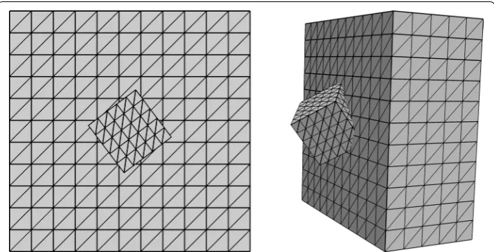
In both cases, the velocity field is divergence free and the right-hand side has been cho-sen to match the given exact solutions. We let the overlapping domain 1 be a d− dimen-sional cube centered in the center of with side length 0.246246 rotated 37° along the z-axis. For d=3, 1 is rotated the same angle along the y-axis as well. The domains i are illustrated in Fig. 6.
The discrete spaces are Pk–Pk−1 Taylor–Hood finite element spaces with
continu-ous piecewise vector-valued polynomials of degree k≥2 discretizing the velocity and discontinuous scalar polynomials of degree l=k−1 discretizing the pressure. These
spaces are inf-sup stable on the uncut elements of the background mesh discretizing 0 and on the whole of 1 and therefore satisfy Assumption B. The linear systems are solved using the direct solver MUMPS, which can be called from FEniCS.
Figures 7 and 8 show the convergence of the error in the H0- and 1 L2-norms in 2D and
3D respectively. Optimal order of convergence is obtained, although limited computer memory resources prevented a study for higher degrees than k=3 in 3D. Note that in this method, the degrees of freedom in the elements in Kh,0∩Ŵ are doubled. Therefore, the total number of degrees of freedom are for this problem comparable to a standard method. In the convergence plots, results for small mesh sizes, roughly corresponding to errors below 10−7 have been removed because errors could not be reliably estimated due to numerical round-off errors in the numerical integration close to the cut cell boundary.
We have not investigated these numerical errors in detail but note that these error norms are notoriously sensitive to compute for small errors and high order. They involve computing an integral of the square of the error, which can be very sensitive to round-off errors since the square (u−uh)2 expands to (u2+u2h)−2uuh, resulting in the subtrac-tion of two “large” numbers of similar size. The computasubtrac-tion is also sensitive to how the exact analytic solution is interpolated into a finite element (of a higher order). For this reason, FEniCS provides a particular function called errornorm, which works around this challenge interpolating u and uh into a common higher order function space1. How-ever, this functionality is not yet supported for the multimesh implementation, so the challenge of large round-off errors in the numerical evaluation of norms remains.
(87) f(x,y)=2π
sin(2πy)(cos(2πx)−2π2cos(2πx)+π2)
sin(2πx)(cos(2πy)+2π2cos(2πy)−π2).
(88) u(x,y,z)=sin(πy)sin(πz)·(1,−sin(πy)cos(πz), sin(πz)cos(πy)),
(89)
p(x,y,z)=πcos(πx),
(90) f(x,y,z)=π2
sin(πsin(2πy)zsin(π)(2 cos(2πz)−sin(πy)−1)x) sin(2πy)(1−2 cos(2πz)
.
Condition numbers
For a numerical study of the algebraic conditioning of the system, we recall the defini-tion of the condidefini-tion number of a matrix A
where σmax(A) and σmin(A) are the maximum and minimum singular values of A. Since
the discrete pressure is only determined up to a constant here, the system matrix A will have one zero singular value. To this end, we take the second smallest singular value when computing the condition number in (91).
There are two issues that need to be address regarding the conditioning of system matrices of interface problems. First, κ should be optimal, i.e. κh−2 (see [3]). Second, the condition number should be essentially independent of the location of the interface. Figure 9 illustrate these properties for the 2D model problem and k=2. Optimal order of convergence is obtained by performing uniform refinement of the two meshes for var-ious values of the Nitsche parameter β (cf. (25)). To investigate the second issue, we set
(91) κ(A)= σmax(A)
σmin(A)
Fig. 6 Location of the overlapping domain in the background mesh. The domain 1 is placed in the center of and rotated along the z-axis in 2D (left) and along the y- and z-axes in 3D (right)
Fig. 7 Convergence results, 2D. A rotated square is embedded in the unit square background mesh. Results in L2 (left) and H1
up the same problem with fixed meshes and shift the center of the overlapping domain in the x direction in steps of 0.0001 until it is shifted 1.25 h. For each mesh configuration we compute κ. This is illustrated in Fig. 9 (right) for various h. The x-axis is normalized with respect to the mesh size: 0 corresponds to the initial position (see Fig. 6) and 1 cor-responds to the overlapping domain being shifted h to the right in the x direction.
Flow around a propeller
To illustrate the method on a complex geometry we create a propeller using the CSG tools of the FEniCS component mshr [22], see Fig. 10 (top left). The lengths of the blades are approximately 0.5. Then we construct a mesh of the domain outside the pro-peller, but inside the unit sphere. This is illustrated in Fig. 10 (top right). The mesh is constructed using TetGen [23] and is body-fitted to the propeller. To simulate the flow around the propeller, the mesh is placed in a background mesh of dimensions [−2, 2]3,
where we have removed the elements with all nodes inside a sphere of radius 0.9, see Fig. 10 (bottom).
The simulation is setup with the inflow condition u(x,y,z)=(0, 0, sin(π(x+2)/4)sin(π(y+2)/4)) at z= −2, the outflow condition
p=0 at z=2 and u(x,y,z)=0 on all other boundaries, including the boundary of the
propeller. The resulting velocity field using degree k=2 is shown in Fig. 11. Note the Fig. 8 Convergence results, 3D. A rotated cube is embedded in the unit cube background mesh. Results in L2 (left) and H1
0 (right) norms
continuity of the streamlines of the velocity going from the finite element space defined on the background mesh to the finite element space defined on the overlapping mesh surrounding the propeller.
Conclusions
We have presented a finite element method for the Stokes problem based on two com-posite meshes that overlap each other. The method is based only on the assumption of
Fig. 10 Propeller geometry and meshes. Propeller geometry (top left) and body-fitted mesh (top right). Non body-fitted background mesh and propeller (bottom)
inf-sup stable polynomial spaces on the two meshes. In fact, the proposed discretiza-tion allows arbitrary inf-sup stable spaces for the Stokes problem to be stitched together using a stabilized Nitsche method from multiple non-matching and intersecting meshes to weakly enforce continuity over an interface. By the use of a least-squares type of sta-bilization, a global inf-sup stable space is constructed. We demonstrate optimal order convergence by both a priori error estimates as well as numerical results for Taylor-Hood elements of polynomial order up to 4. The method has several practical applica-tions and one such prime example is the discretization of flow around complex objects. Future work includes the extension to time-dependent problems and to fluid–structure interaction.
Authors’ contributions
All authors contributed to the development of the theory. The computer code for the numerical simulations was devel-oped by AJ and AL. All authors read and approved the final manuscript.
Author details
1 Center for Biomedical Computing, Simula Research Laboratory, P.O. Box 134, 1325 Lysaker, Norway. 2 Department of Mathematics and Mathematical Statistics, Umeå University, 90187 Umeå, Sweden. 3 Department of Mathematical Sci-ences, Chalmers University of Technology and University of Gothenburg, 41296 Göteborg, Sweden.
Acknowledgements
This research was supported in part by the Swedish Foundation for Strategic Research Grant No. AM13-0029, the Swedish Research Council Grant No. 2013-4708, and the Swedish Research Council Grant No. 2014-6093. The work was also supported by The Research Council of Norway through a Centres of Excellence grant to the Center for Biomedical Computing at Simula Research Laboratory, project number 179578.
Compliance with ethical guidelines Competing interests
The authors declare that they have no competing interests.
Received: 2 May 2015 Accepted: 12 August 2015
References
1. Nitsche J. Über ein Variationsprinzip zur Lösung von Dirichlet-Problemen bei Verwendung von Teilräumen, die keinen Randbedingungen unterworfen sind. Abh Math Sem Hamburg. 1971;36:9–15.
2. Hansbo A, Hansbo P, Larson MG. A finite element method on composite grids based on Nitsche’s method. ESAIM-Math Model Num. 2003;37(3):495–514. doi:10.1051/m2an:2003039.
3. Massing A, Larson MG, Logg A, Rognes ME. A stabilized Nitsche overlapping mesh method for the Stokes problem. Numer Math. 2014;128(1):73–101. doi:10.1007/s00211-013-0603-z.
4. Massing A, Larson MG, Logg A. Efficient implementation of finite element methods on nonmatching and overlap-ping meshes in three dimensions. SIAM J Sci Comput. 2013;35(1):23–47. doi:10.1137/11085949X.
5. Hansbo P, Larson MG, Zahedi S. A cut finite element method for a Stokes interface problem. Appl Numer Math. 2014;85:90–114. doi:10.1016/j.apnum.2014.06.009.
6. Chesshire G, Henshaw WD. Composite overlapping meshes for the solution of partial differential equations. J Com-put Phys. 1990;90(1):1–64. doi:10.1016/0021-9991(90)90196-8.
7. Benek JA, Buning PG, Steger JL. A 3-D chimera grid embedding technique. Technical Report 85–1523, AIAA (1985). 8. Houzeaux G, Codina R. A Chimera method based on a Dirichlet/Neumann(Robin) coupling for the Navier-Stokes
equations. Comput Method Appl M. 2003;192(31–32):3343–77. doi:10.1016/S0045-7825(03)00276-7. 9. Gerstenberger A, Wall WA. An eXtended Finite Element Method/Lagrange multiplier based approach for
fluid-structure interaction. Comput Method Appl M. 2008;197(19–20):1699–714. doi:10.1016/j.cma.2007.07.002. 10. Shahmiri S, Gerstenberger A, Wall WA. An XFEM-based embedding mesh technique for incompressible viscous
flows. Int J Numer Meth Fl. 2011;65(1–3):166–90. doi:10.1002/fld.2471.
11. Brezzi F, Fortin M. Mixed and hybrid finite element methods. New York: Springer; 1991.
12. Arnold DN, Brezzi F, Cockburn B, Marini LD. Unified analysis of discontinuous Galerkin methods for elliptic problems. SIAM J Numer Anal. 2002;39(5):1749–79. doi:10.1137/S0036142901384162.
13. Boffi D, Brezzi F, Fortin M. Mixed finite element methods and applications. Berlin Heidelberg: Springer; 2013. 14. Scott LR, Zhang S. Finite element interpolation of nonsmooth functions satisfying boundary conditions. Math
Comp. 1990;54:483–93. doi:10.1090/S0025-5718-1990-1011446-7.
16. Arnold DN, Brezzi F, Fortin M. A stable finite element for the Stokes equations. Calcolo. 1984;21(4):337–44. doi:10.1007/BF02576171.
17. Braess D. Finite elements: theory, fast solvers, and applications in solid mechanics. Cambridge: Cambridge University Press; 2007.
18. Verfürth R. Error estimates for a mixed finite element approximation of the Stokes equation. RAIRO Anal Numer. 1984;18:175–82.
19. Brenner SC, Scott LR. The mathematical theory of finite element methods. New York: Springer; 2008.
20. Logg A, Mardal K-A, Wells GN, et al. Automated solution of differential equations by the finite element method. Berlin Heidelberg: Springer; 2012.
21. Logg A, Wells GN. DOLFIN: automated finite element computing. ACM Trans Math Soft. 2010. doi:10.1145/1731022.1731030..
22. Kehlet B. mshr: Mesh generation component of FEniCS. https://bitbucket.org/benjamik/mshr (Accessed: 2015-01-08).