Factors Affecting Health Insurance Premiums: Explorative and Predictive Analysis Creative Component Project Report

Creative Components Iowa State University Capstones, Theses and _{Dissertations}

Fall 2018

Factors affecting health insurance premiums: Explorative and

Factors affecting health insurance premiums: Explorative and

predictive analysis

predictive analysis

Tarunpreet Kaur

Iowa State University, [email protected]

Follow this and additional works at: https://lib.dr.iastate.edu/creativecomponents

Part of the Business Analytics Commons, and the Insurance Commons

Recommended Citation Recommended Citation

Kaur, Tarunpreet, "Factors affecting health insurance premiums: Explorative and predictive analysis" (2018). Creative Components. 72.

https://lib.dr.iastate.edu/creativecomponents/72

1

Factors Affecting Health Insurance Premiums:

Explorative and Predictive Analysis

Creative Component Project Report

By

Tarunpreet Kaur

Master of Science in Information Systems

Submitted in fulfilment for the requirements for the degree of

Master of Science in Information Systems

Major Professor:

Dr. Zhengrui Jiang

Ivy College of Business

Iowa State University

Ames, Iowa

2

TABLE OF CONTENTS

ACKNOWLEDGEMENT ... 5

ABSTRACT ... 6

PROJECT GOALS AND MOTIVATION ... 7

DATA DESCRIPTION ... 8

PROJECT METHODOLOGY AND DESIGN ... 10

DATA PREPROCESSING ... 12

EXPLORATORY DATA ANALYSIS (EDA) ... 13

PREDICTIVE MODELLING ... 17

MEASURING MODEL PERFORMANCE ... 18

PREDICTIVE MODELS ... 19

MODEL 1- MULTIPLE LINEAR REGRESSION ... 19

MULTIPLE LINEAR REGRESSION APPLIED TO THE DATASET ... 20

MODEL 2 – RANDOM FOREST ... 22

RANDOM FOREST APPLIED TO THE DATASET ... 23

MODEL 3 – NEURAL NETWORK ... 26

NEURAL NETWORK APPLIED TO THE DATASET ... 27

SUMMARY OF MODEL COMPARISON ... 29

CONCLUSION ... 31

3

LIST OF FIGURES

Figure 1: Diagram of dependent and independent variables………10

Figure 2: Methodology Approach……….11

Figure 3: Data Analysis Steps………12

Figure 4: Scatterplot of Charges and Age/BMI………...13

Figure 5: Scatterplot of Charges and Age/BMI based on smoker………...14

Figure 6: Scatterplot of Charges and Sex/ No. of Children………...15

Figure 7: Scatterplot of Charges and Smoker/Region………...16

Figure 8: Steps OF Predictive Modelling………..17

Figure 9: Plot of Actual vs. Predicted values for multiple linear regression model………..21

Figure 10: Corresponding RMSE and mtry values for random forest………...24

Figure 11: Plot of Actual vs. Predicted values for random forest model………...25

Figure 12: Schematic diagram of a neural network………...26

Figure 13: Corresponding values of hidden units and RMSE………...27

Figure 14: Plot of Actual vs. Predicted values for neural network model……….28

4

LIST OF TABLES

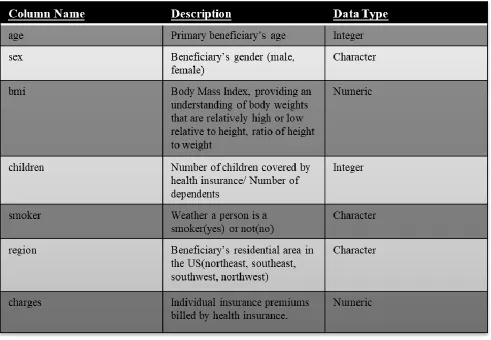
Table 1: Description of columns and its data-types………9

Table 2: Metric values for multiple linear regression………....20

Table 3: Metric values for random forest model………...23

Table 4: Metric values neural network model………...27

5

ACKNOWLEDGEMENT

I would like to acknowledge Dr. Zhengrui Jiang, my major professor. This project would not have

been possible without his constant support and guidance from the beginning till the end. I am

highly indebted to him.

I would also like to extend my gratitude to my family, friends and peers. Additionally, I would

also like to thank the graduate department faculty, other professors whose classes I have taken a

and learned a lot from them and staff for making my time at Iowa State University a wonderful

and an enriching experience.

I have learned a lot during my master’s journey at Iowa State University and look forward to

6

ABSTRACT

The main foundational block of health insurance industry is to estimate the future events and

measure the associated risk/value of these events, hence it is needless to say that predictive

analytics is used widely to determine the risk, insurance premium and enrich overall customer

experience.

The health insurance industry has always been a slow-moving industry when it comes to adopting

the data analytics practices into its business models. With the advent of advanced data analytics

technologies, it has become important more than ever to take advantage of such sophisticated

analytics to accurately assess and predict the insurance premiums for the insured.

Thus, one of the important tasks for health insurance companies is to determine the policy

premiums. By using predictive modelling, the insurers can determine the policy premium for the

insured based on their behaviors which are indicated by attributes such as age, BMI (Body Mass

Index), smoking habits, number of children etcetera.

This determination of premiums based on the data collected for an individual helps insurance

companies in enhanced pricing, underwriting and risk selection. Additionally, it helps in making

better decisions, understanding customer needs and be fair to the customers. Acquiring a

comprehensive understanding of customer behaviors and habits from historical data helps insurers

7

PROJECT GOALS AND MOTIVATION

Judicious use of predictive analysis has empowered health insurers to improve their premium

pricing accuracy, create customized health insurance plans and services, and build stronger

customer relationships.

Thus, the main goal of this project is to predict the insurance premiums based on the behavioral

data collected from the individuals so that insurance companies can make useful and accurate

predictions.

Based on these predictions, they can then evaluate the following decisions and make better

judgement calls:

• Which individuals deserve which kind of insurance plan?

• Based upon an individual’s behavior, predicting their premium helps in better risk

8

DATA DESCRIPTION

The dataset is originally from the book called Machine Learning with R by Brett Lantz. The dataset

is however made available online through the GitHub repository called Machine Learning with R.

This dataset contains the information on individual attributes such as sex, age, smoking habits

etcetera. It has:

• 1338 rows

• 7 columns

Description of columns:

➢ age – age of primary beneficiary

➢ sex – gender of the beneficiary. It has two categories:

o Male

o Female

➢ bmi – Body Mass Index, providing an understanding of body weights that are relatively

high or low relative to height, objective index of body weight (kg/m^2) using the ratio of

height to weight, ideally 18.5 to 24.9

➢ children – Number of children covered by the health insurance / Number of dependents.

➢ smoker – describing whether a person is a smoker or a non-smoker. It has 2 values:

o Yes

o No

➢ region – the beneficiary’s residential area in the US. It has 4 region values:

o Northeast

9 o Southwest

o Northwest

➢ charges – Individual insurance premiums billed by health insurance.

10

PROJECT METHODOLOGY AND DESIGN

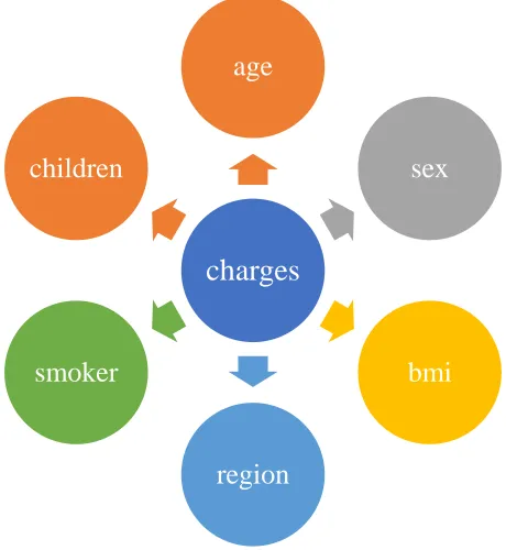
The main goal of the project is to predict the insurance premium charge based upon other

attributes.

The dependent variable is charge.

There are 6 independent variables:

✓ age

✓ sex

✓ children

✓ bmi

✓ smoker

✓ region

The following figure shows the independent and dependent variables:

Figure 1 – Diagram of dependent and independent variables

charges

age

sex

bmi

region smoker

11

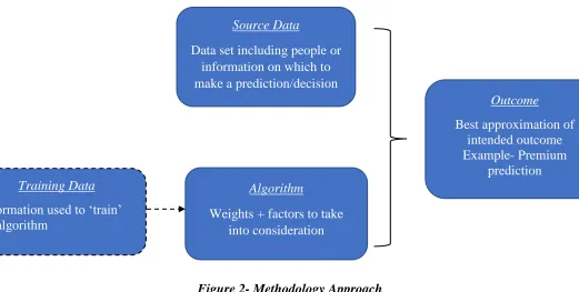
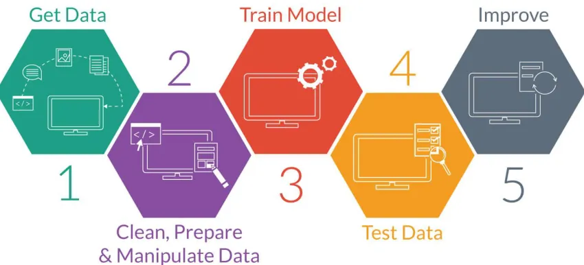
The following steps are followed for the methodology approach:

➢ Data is downloaded as .csv file.

➢ Data is analyzed, cleaned and manipulated according to desired algorithm application.

➢ Exploratory Data Analysis (EDA) is performed to see the effect of each independent

variable on the dependent variable.

➢ Based upon the EDA, the following machine learning models are selected:

• Multiple Linear Regression

• Random Forest

• Neural Network

➢ The models are evaluated against each other to find the best one.

The following figure represents the high-level methodology and design approach used:

Figure 2- Methodology Approach

Training Data

Information used to ‘train’ an algorithm

Source Data

Data set including people or information on which to make a prediction/decision

Algorithm

Weights + factors to take into consideration

Outcome

Best approximation of intended outcome Example- Premium

12

DATA PREPROCESSING

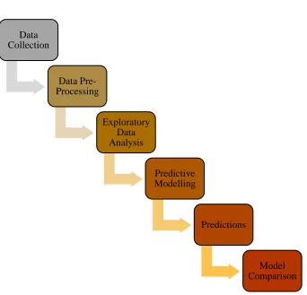
The following steps illustrate the steps of data pre-processing:

➢ Columns sex, region, smoker are converted to categorical variables first and then were

converted to numerical variables to be compatible with the model building.

➢ Missing values are removed, and the data is cleaned for analysis and model building.

➢ Some columns are scaled for the model building.

➢ 5- cross validation is performed to train and test the data and compute the out-of-sample

metrics.

Steps of data analysis:

13

EXPLORATORY DATA ANALYSIS (EDA)

The relationship between all the independent variables and the dependent variable are explored

in the initial exploratory data analysis phase.

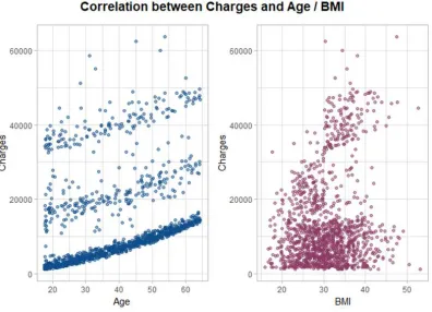
The following figure depicts the relationship between age and BMI.

Figure 4 – Scatterplot of Charges and Age/BMI

A scatterplot is created to show these relationships:

For age, the relationship is almost linear as the charges increase with increase in the age of the

person.

However, for BMI the relationship does not seem to be linear. Nevertheless, charges increase with

14

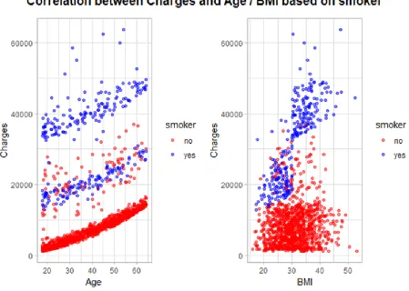
Figure 5 – Scatterplot of Charges and Age/BMI based on smoker

Even for the same age group, charges are higher for a person who smokes than a non-smoker as

shown by the blue (person who smokes) and red (person who does not smoke) dots.

15

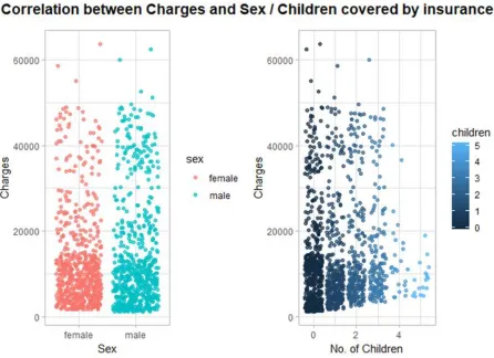
To examine the relationships between the columns sex and children, the scatterplot is used.

The following figure depicts that no significant relationship exists between the gender od a

person and the premium charges.

However, it can be seen that the charges increase with increase in the number of children.

16

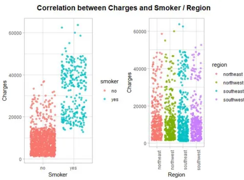
The following figure illustrates that charges are significantly higher for smokers as compared to

non-smokers.

On the other hand, it can be seen that region does not seem to have any relationship with the

charges i.e. people living in the different residential areas of northeast, northwest, southeast and

southwest have almost no difference in the charges.

17

PREDICTIVE MODELLING

Predictive Modelling is the process of uncovering relationships within the data by using a

mathematical model for predicting some desired outcome. It uses historical data to make

predictions about unseen data.

The following figure depicts the cycle of the predictive modelling:

Figure 8- Steps OF Predictive Modelling

The goal is to predict the premium charge which is a numeric outcome. So, regression models

like multiple linear regression, random forest and neural networks are used for predictive

18

MEASURING MODEL PERFORMANCE

For measuring the performance of the regression models, following metrics have been used:

➢ Root mean squared error (RMSE) – This is a function of the residuals where residuals

are the difference between the predicted values and observed/actual values:

residuals = observed – predicted

Using residuals, we then calculate the mean squared error (MSE) which is computed by

squaring the residuals, summing them and dividing by the number of samples.

MSE =

2

𝑛

where n is the number of samples.

RMSE is then calculated by taking a square root of the MSE so that it is in the same units

as original data:

RMSE =

√

𝑛

The value of RMSE tells us approximately how far away (on average) the predictions are

from true values.

➢ Coefficient of Determination(R-squared) – This value can be interpreted as the

proportion of variability in the response(dependent) variable that is explained by the model.

It is calculated by squaring the correlation coefficient between the observed and predicted

19

PREDICTIVE MODELS

As mentioned earlier, to predict the premium charge, three predictive models have been used and

compared against each other. Each model is explained in detail in the following pages:

➢ Multiple Linear Regression

➢ Random Forest Regression

➢ Neural Network

MODEL 1- MULTIPLE LINEAR REGRESSION

Multiple linear regression model is used to predict a numeric outcome (dependent variable) based

on two or more independent variables. We assume that the value of the response/dependent

variable is some function of the explanatory variables and some random noise. The generic

statistical model equation is:

Response = f(explanatory) + noise

The model generally takes the following form:

𝑦 = 𝛽𝜊 + 𝛽1𝑥1+ 𝛽2𝑥2+ ⋯ + 𝛽𝑘𝑥𝑘+ 𝜀

where y is the dependent variable and 𝑥₁, 𝑥₂, … . . 𝑥_𝑘 are independent variables and 𝜀 is the

random-error term(noise) and has normal distribution with mean = 0 and fixed standard deviation:

𝜀 ∽ 𝑁(0, 𝜎𝜖)

The value of the coefficient 𝛽_𝑖 determines the contribution of the independent variable 𝑥_𝑖 and 𝛽𝜊

is the y-intercept which tells the value of the dependent variable when the values of all the

independent variables is zero.

Advantages of Multiple linear regression:

20 • It is easily interpretable.

• Ability to identify outliers or anomalies.

Disadvantages of Multiple linear regression:

• They are useful only when the relationship between independent and dependent variable is

linear in nature.

• They cannot effectively be used to capture non-linear relationships between dependent and

independent variables

MULTIPLE LINEAR REGRESSION APPLIED TO THE DATASET

Multiple linear regression is applied to the dataset and the following results are generated.

5-fold cross validation is created to generate the out of sample metrics of RMSE and R-squared:

Table 2 – Metric values for multiple linear regression

The RMSE is 0.0971 and R-squared is 0.7513

The coefficients for different variables were obtained as follows:

age: 0.188

sex: -0.002

bmi: 0.197

children: 0.038

smoker: 0.38

21

Thus, it can be concluded that sex and region does not have a positive relationship with the

charges where as smoker has the highest impact on the charges followed by bmi and age.

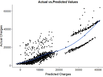
PLOT OF ACTUAL VS. PREDICTED VALUES FOR MULTIPLE LINEAR

REGRESSION MODEL

This figure shows the actual charges versus the predicted charges and the regression line which

shows how well the multiple linear regression model fits the data.

22

It can be seen that although the model performed well for the charges that fall under lower bracket,

it did not do a great job of predicting the values for higher charges. The blue line is the regression

line for the linear model.

MODEL 2 – RANDOM FOREST

One of the disadvantages of multiple linear regression is that it cannot appropriately capture

non-linear relationships between the dependent and independent variables. To overcome this problem,

an ensemble method called Random Forest is used to predict the outcome. Random Forest is an

ensemble method that combines many decision trees to predict the value of the outcome. Each

tree(model) in the ensemble is used to generate a prediction for a new random sample and these m

predictions are averaged to give the forest’s prediction. The algorithm randomly selects the number

of predictors at each split.

Random forest’s tuning parameter is the number of predictors to be selected randomly at each split

and this number is called mtry.

ADVANTAGES OF RANDOM FOREST

• Effectively capture the non-linearity between the response and explanatory variables as

compared to multiple linear regression models.

• They can effectively handle many types of predictors (categorical, continuous, skewed,

etc.) without the need to pre-process them.

• It does not require the user to explicitly specify the form of the predictor’s relationship to

23

DISADVANTAGES OF RANDOM FOREST

• Model instability – minor changes in data can significantly alter the tree’s structure

resulting in inaccurate interpretations.

• They become highly computational as the number of trees increases.

• They can sometimes lead to overfitting

RANDOM FOREST APPLIED TO THE DATASET

Random forest is applied to the dataset and the following results are generated.

5-fold cross validation is created to generate the out of sample metrics of RMSE and R-squared:

Optimal value for mtry selected is 6 based upon the least RMSE of 0.074.

24

The following figure shows different values of mtry and corresponding values of RMSE

25

PLOT OF ACTUAL VS. PREDICTED VALUES FOR RANDOM FOREST MODEL

This figure shows the actual charges versus the predicted charges and the regression line which

shows how well the random forest model fits the data.

Figure11 - Plot of Actual vs. Predicted values for random forest model

For the random forest model, it can be seen from the above figure that this model performed

better as compared to the multiple linear model as the blue regression line is fitting the charge

26

MODEL 3 – NEURAL NETWORK

Neural Networks are powerful non-linear regression techniques inspired by theories about how the

brain works. The outcome is modeled by an intermediary set of unobserved variables (called

hidden variables or hidden units).

These hidden units are linear combinations of the original predictors

27

NEURAL NETWORK APPLIED TO THE DATASET

Neural network is applied to the dataset and the following results are generated.

5-fold cross validation is created to compute the out of sample metrics of RMSE and R-squared:

Optimal value for the number of hidden layers selected is 1 with 5 nodes based upon the least

RMSE of 0.072.

Table 4- Metric values neural network model

The following figure shows the number of hidden units in layer 1 of the neural network and the

corresponding values of RMSE.

28

PLOT OF ACTUAL VS. PREDICTED VALUES FOR NEURAL NETWORK MODEL

This figure shows the actual charges versus the predicted charges and the regression line which

shows how well the neural network model fits the data.

Figure 14 - Plot of Actual vs. Predicted values for neural network model

The above figure shows that for the neural network model, the blue regression line is fitting very

well as compared to the two other model as previously discussed.

Thus, the neural network model performed significantly better than the random forest and linear

29

SUMMARY OF MODEL COMPARISON

Out of the 3 models: multiple linear regression, random forest and neural network, the neural

network performed the best with the least RMSE of 0.072 and highest R-squared of 0.859.

The following table compares the RMSE and R-squared of the 3 models.

Table 5 – Metric Comparison for the three models

The neural network has done a better job of predicting the insurance charges because neural

network is an advanced machine learning algorithm that captures the complex interactions between

the independent variables as compared to the simpler algorithms such as multiple linear regression

and random forest regression.

The more a model captures these complex interactions between the variables, the better it performs

and results in predictions that are closer to the actual values.

The figure on the next page shows the actual versus predicted values of the 3 models. Again, we

can see that the neural network performed the best:

30

Figure 15- Actual vs. Predicted plot comparison for three models

MULTIPLE LINEAR REGRESSION

RANDOM FOREST

31

CONCLUSION

Based on the findings of the project, it can be said that predictive modeling has tremendous benefits

for the health insurance industry in determining how much the premium should be charged to the

insured based upon his/her behaviors and health habits. Health insurance companies can then

accurately charge the premium based upon a specific individual’s attributes.

This will not only help the individuals in getting charged the right amount of premium for their

health insurance but will also help in forging better relationships and a level of trust between the

insurance company and the insured.

Based on these predictions, the health insurance providers can then evaluate the following

decisions and make better judgement calls:

✓ Which individuals deserve which kind of insurance plan?

✓ How much the premium should be charged based on an individual’s behaviors?

✓ Based upon an individual’s behavior, predicting their premium helps in better risk

management.

✓ It helps forge trust between the customer and the insurance company.

Thus, it is important for a health insurance company to collect and analyze the data such

as a person’s age, BMI, health data to accurately predict the risk and charge accurate

premiums to cover that risk.

However, there are certain limitations which is the scope of further studies. The data did not

include any information on an individual’s medical costs, the real-time data i.e. data collected from

the sensors in the wearable health devices such as fit bits etcetera. If we take all these types of

different data sources into account then we can have a better picture of an individual’s behavior

32

REFRENCES

1. Nyce, Charles (2007), Predictive Analytics White Paper(PDF), American Institute for

Chartered Property Casualty Underwriters/Insurance Institute of America

2. Conz, Nathan (September 2, 2008), "Insurers Shift to Customer-focused Predictive

Analytics Technologies", Insurance & Technology

3. Rencher, Alvin C.; Christensen, William F. (2012), "Chapter 10, Multivariate regression

– Section 10.1, Introduction", Methods of Multivariate Analysis, Wiley Series in

Probability and Statistics, 709 (3rd ed.), John Wiley & Sons, p. 19, ISBN9781118391679.

4. "Linear Regression (Machine Learning)" (PDF). University of Pittsburgh.

5. Ho, Tin Kam (1995). Random Decision Forests (PDF). Proceedings of the 3rd

International Conference on Document Analysis and Recognition, Montreal, QC, 14–16

August 1995. pp. 278–282. Archived from the original (PDF) on 17 April 2016.

Retrieved 5 June 2016.

6. Liaw A (16 October 2012). "Documentation for R package randomForest" (PDF).

Retrieved 15 March 2013.

7. "Artificial Neural Networks as Models of Neural Information Processing | Frontiers

Research Topic". Retrieved 2018-02-20.

8. Hoskins, J.C.; Himmelblau, D.M. (1992). "Process control via artificial neural networks

and reinforcement learning". Computers & Chemical Engineering. 16 (4): 241–

251. doi:10.1016/0098-1354(92)80045-B.