Engineering III Mac Eng Class of 2015

C

HAPTER

3:

S

TEADY

S

TATE

1-D

C

ONDUCTION

We already mentioned the parallels between heat flow and electrical

current flow and the idea of k and h

being measures of the resistance to heat transfer through a medium

For electricity, resistance is related to the flow (of electrons) by Ohm’s Law:

In parallel, for heat flow:

_R

T

q

=

∆

We will generate expressions for

thermal resistance R in different cases Voltage – Driving Force

R

V

I

=

Electrical Resistance to Flow

Temperature Difference - Driving Force

Thermal Resistance to Flow Flow (of

electrons)

Flow (of heat)

Conduction Through Plane Walls In general: = +             ∂ ∂ ∂ ∂ +       ∂ ∂ ∂ ∂ +       ∂ ∂ ∂ ∂ q z T k z y T k y x T k

x & _t

T c_p

∂ ∂

ρ

For a slab or wall at steady state with no internal heat generation (applying the semi-infinite assumption)

_ = 0

          ∂ ∂ ∂ ∂ x T k

x ! 2 0

2 = ∂ ∂ x T

if k=constant

Integrating this expression:

T(x) = C1x + C2

" y=mx+b – linear T profile inside slabs with no heat generation

Since q = −kA∂_∂T_x , therefore q = −kAC1

where C1=slope of temp. profile

If C1 is the slope,

x

T

x

x

T

T

C

∆

∆

=

−

−

=

1 2

1 2

1

So, q = −kA ∆_∆T_x = ∆_RT

Thus, thermal resistance is defined as

R = ∆_kAx (slab, 1-D, steady state) We could also get this result by

applying our boundary conditions: In general, T(x) = C1x + C2

B.C. #1 – Dirichlet - T=T1 at x=0

! T1=C1(0)+C2 ! T1= C2

B.C. #2 – Dirichlet - T=T2 at x=L

! T2=C1L+C2 = C1L+T1

C T _LT T_x

∆ ∆

=

−

= 2 1 1

x

T₁

T2

qx

L

Conduction Through Cylinders

For a tube or hollow cylinder, it is harder to give an equation since the semi-infinite assumption may not hold i.e. the axis over which the heat flow is occurring may be different

Radial flow is most common:

0 1

=

   

 

   

 

∂ ∂ ∂

∂

r T kr r

r (no heat generation)

if k is constant _ = 0

 

 

   

 

∂ ∂ ∂

∂

r T r r

Integrating, C1 r

T

r  =

  

 

∂ ∂

, _r

C r

T ₁

=

   

 

∂ ∂

Therefore, the temperature profile is:

2

1 lnr C

C

T = +

Thus, in a cylinder, the temperature profile is logarithmic over the radius.

Applying boundary conditions:

T = Ti @ r = ri

T = To @ r = ro

Solve for C1, C2 via

substitution:       − = o i o i r r T T C ln 1

(

) ( )

      − −       = o i i o i o i i r r r T T r r T C ln ln ln 2

Substituting into T = C1 ln r + C2 :

o o i o o i T r r r r T T T +             − = ln ln ) (

or _

           = − − o i o o i o r r r r T T T T ln ln

and _

     − = ∂ ∂ o i o i r r T T r r T ln 1

(since d/dx(ln ax)=1/x) r_o

r_i Ti To r_o

r_i Ti To

For a cylinder, the rate of heat flow is:

_r

T

r

kA

q

∂

∂

−

=

(

)

A(r)=radial cross-sectional area= 2πrL

Therefore,

(

)

_r

T

rL

k

q

∂

∂

−

=

2

π

Substituting dT/dr:

_











−

⋅

−

=

i o

o i

r

r

T

T

kL

q

ln

2

π

Again in parallel to Ohm’s Law, with q

as the flow term and ∆T = Ti – To as

the driving force, the measure of

thermal resistance for this example is:

(cylinder, 1D radial, steady state)

Q: What if ri = 0?

kL

r

r

R

i

o

π

2

ln













=

Conduction Through Spheres

For a hollow sphere, again it is harder to give an equation since the

semi-infinite assumption may not hold

i.e. the axis over which the heat flow is occurring may be different

Again, radial flow is most common:

0

1

₂

2



=























∂

∂

∂

∂

r

T

kr

r

r

(no heat generation)

For constant k: 2 _ = 0

 

 

   

 

∂ ∂ ∂

∂

r T r

r

Thus, 1

2

C r

T

r  =

  

 

∂ ∂

and 2

1

1r C

C

T = − +

B.C. T = Ti @ r = ri ! 2 1

1r C

C

T_i = _i− +

B.C. T = To @ r = ro ! 2 1

1r C

C

T_o = _o− +

Combining, 1 1 1 1 − −

−

=

−

_{i o o}

i

C

r

T

C

r

T

Rearranging,

(

)













−

−

=

o i o i

r

r

T

T

C

1

1

1 Substituting,

(

)

2 1 1

1 r C

r r T T T o i o i +                   − − =

Using B.C. T = To @ r = ro again to

solve for C2 and substituting, we get,

o r r r r o

i

T

T

T

T

o i o

+

−

−

−

=

1 1 1 1

)

(

or o i o r r r r o i o

T

T

T

T

1 1 1 1

−

−

=

−

−

and

(

)

(

)

1

1 1

2 i o

r r

T

T

r

r

T

o i

−

−

−

=

δ

δ

For a sphere, the heat flow rate is:

r

T

r

kA

q

∂

∂

−

=

(

)

A(r) = radial cross-sectional area = 4πr2

Therefore,

(

)

_r

T

r

k

q

∂

∂

−

=

4

π

2

Substituting dT/dr,

[

]

o i r

r

o

i

T

T

k

q

1 1

4

−

−

=

π

Again in parallel to Ohm’s Law, with q as the flow term and ∆T = Ti – To as

the driving force, the measure of

thermal resistance for this example is:

(sphere, 1D radial, steady state)

[

]

k

R

ri ro

π

4

1 1

₋

=

Just as with conduction, we can derive resistive terms to express heat

transfer for convection and radiation

Convection:

q

=

hA

(

T

s

−

T

∞

)

Therefore,

_q

_hA

T

T

R

=

s

−

∞

=

1

Radiation:

q

rad

=

h

r

A

(

T

s

−

T

surr

)

where

h

r

=

εσ

(

T

s

+

T

surr

)

(

T

s2

+

T

surr2

)

Therefore,

_q

_h

_A

T

T

R

r

s

−

₌

1

=

∞

NOTE: hr is not a true heat transfer

coefficient but represents a grouped,

T-sensitive term which allows us to linearize the radiation equation

R

T

q

=

∆

R

T

q

=

∆

Contact Resistance at Joints:

In the real world, surfaces are NEVER smooth, so when two objects are

pressed together, there will be an

irregular gap filled with air, oil, etc. " also: adhesives, joints, welds

The temperature profile is therefore discontinuous – there is a thermal contact resistance (Rtc).

See Tables 3.1,3.2

NOTE: text values are per unit area

(Rtc”) and thus represent 1/hc

A

h

q

T

T

R

c B

A tc

1

=

−

=

Temp. Profile

Summary of Resistance Terms (all terms should be in units K/W)

Conduction: 1D, steady (Table 3.3)

kA

x

R

=

∆

_kL

r

r

R

i

o

π

2

ln













=

[

]

k

R

ri ro

π

4

1 1

₋

=

Wall/slab Cylinder Sphere

Convection:

_q

_hA

T

T

R

=

s

−

∞

=

1

Radiation:

_q

_h

_A

T

T

R

r

s

−

₌

1

=

∞

Contact:

So… How do these equations help us solve heat transfer problems?

A

R

A

h

q

T

T

R

tc

c B

A tc

"

1

=

=

−

=

E

QUIVALENT

T

HERMAL

C

IRCUITS

Electric circuits can be analyzed as a series of resistive elements

Resistors in series Total resistance =

sum of resistances

R1 + R2 + R3 = Rtotal

Resistors in parallel Total resistance =

reciprocal sum of resistances

total

R

R

R

R

1

1

1

1

3 2

1

=

+

+

The same method can be used to solve heat flow problems (but NOT temperature distribution problems)

R3

R1

R2

R1

R1 R2 R3

Consider the analogy with fluid flow:

Flow=Pressure Gradient (driving force)

Frictional Drag (resistance) Q: Compare the resistance in the following scenarios (hollow tubes):

(a)

(b)

(c)

(d)

(e)

Answer:

Using (a) as the reference case

Resistance in flow direction

(b) decrease tube length decrease

total friction from fluid decrease resistance ( )

(c) decrease tube diameter increase % of fluid in contact with wall

increase friction, resistance ( )

(d) fluid experiences 1/2 friction of (a) + 1/2 friction of (b) add friction

(e) fluid can distribute between large d (lower friction, higher flow) and small d (higher friction, lower flow)

tubes more fluid flows

EXAMPLE 1: Glass window at steady state, with convective heat transfer inside and outside and conduction

through the glass – find the heat flow:

We can solve this problem directly using conservation of energy i.e.

q(out) of any layer must equal q(in):

A

h

T

T

A

k

x

T

T

A

h

T

T

q

o

o o

s

glass o s i

s

i

i s i

x

1

1

, ,

, ,

,

, ∞

∞

−

=

∆

−

=

−

=

Need to know at least one surface temperature to solve the problem

Instead, write an equivalent thermal circuit accounting for each of these heat transfer events:

Thus, we can reduce the problem to a set of resistors in series, such that the total heat transfer resistance is:

_kA

_h

_A

L

A

h

R

o i

total

1

1

+

+

=

and the total heat flow is:

_total

o i

x

R

T

T

q

=

∞,

−

∞,

Ignore temperatures in the interior of circuit

system of equations ! simple algebra 1/hiA

1/hoA L/kA q

EXAMPLE 2: Heat flows from left to right in the composite material below

q

A k

L

A

A k

( )

A

L

B B

3 2

A B

C

D

( )

A k

L

C C

3 1

A k

L

D D

Q: How will the heat get distributed between materials B and C?

In this case, the heat transfer is a

combination of units in series (A,B/C, and D) and parallel (B and C)

q

L

2/3y

1/3y

Insulation

( )

( )

∑

+ +

  

 

  

 

+ =

=

−

A k

L

A k

L

A k

L A

k L R

R

D D

A A

C C B

B t

tot

1

3 1 3

2

1 1

Q: What would happen in this case?

One branch

of the circuit One branch of the circuit

q

L

2/3y

1/3y

A B C

D

E

Insulation

EXAMPLE 3: Critical Insulation

A pipe with containing stationary hot water at Tw is insulated using a layer

of foam. Find the heat flow through the insulation as a function of the radius and the insulation thickness which gives the maximum heat flow.

Do the heat analysis using both heat balances and equivalent circuits.

ho, T∞

rp

ri

ro

Tp

Ti

To

ANSWER:

Heat Balances

Water at rest: Tw = Tp (no convection)

Conduction through pipe: Conduction through insulation: Convection from outer surface:

Add all equations – inner T cancel:

(

)

_      +       + = ∞ − p i i o o o w r r kL q r r kL q L r h q T T ln 2 1 ln 2 1 2 1 π π π

(

r

L

)

h

kL

r

r

kL

r

r

T

T

q

o o i o p i w

π

π

π

2

1

2

ln

2

ln

+













+













−

=

∞

















=

−

p i i p

r

r

kL

q

T

T

ln

2

1

π

(

r

L

)

Equivalent Circuits:

(

r

L

)

h

kL

r

r

kL

r

r

T

T

R

T

T

q

o o i o p i w total w x

π

π

π

2

1

2

ln

2

ln

+













+













−

=

−

=

∞ ∞

! same as heat balance approach!

qtotal Tw

Ti T_o

T∞ kL r r p i π 2 ln       kL r r i o π 2 ln       hA 1

pipe insulation surface

To maximize q, we must minimize the denominator by changing ro:

0

=

o

dr

dq

(condition for maximization)

( )

_o

o i o p i w x

r

h

k

r

r

k

r

r

L

T

T

q

1

ln

ln

1

)

2

)(

(

+













+













−

=

_∞

π

( )

0 1 ln ln 1 ) 2 )( ( =                   +       +       − = _∞ o o i o p i o w o r h k r r k r r dr d L T T dr dq π

Cancelling the constant terms and taking the derivative (quotient rule):

0

1

1

1

2

=

−

o o

hr

r

k

!

_h

k

r

_o,crit

=

What does this result mean?

Heat flow through an insulating layer has a maximum at a thickness ro

Why? This rather unexpected result is due to the fact that the addition of

insulation significantly increases the effective (outside) heat transfer area of small cylinders (i.e. wires)

" Applied to cool high voltage power transmission wires

Typical value, ro,crit ~ 0.05/5 = 1 mm

q

r

r

i

r

_o,

T

HERMAL

C

IRCUITS

W

ITH

H

EAT

I

NPUTS

If a thermal circuit includes a heat

generating element, add that element into the circuit and perform an energy balance at the point of generation

EXAMPLE: Rear window of an

automobile with a thin film heater on the inside and a tinted layer on the outside. Draw the thermal circuit and find the electrical power required to keep the inside surface at 15°C

Inside air

T∞,i = 25°C

hi = 65W/m2K

Ts,i = 15°C

Window Lw=0.01m

kw = 1.4W/mK

Thin heater

qh”

Tinted Window

Ltw = 0.002m

ktw = 0.5W/mK

Outside air

T∞ = -10°C

ho = 100W/m2K

Q: What if the contact resistance between the non-tinted and tinted

glass was not negligible? Rewrite the thermal circuit and heat balance

equation using resistance theory.

A: Thermal Circuit:

Heat Balance:

A h_i

1

T∞,i

q”h

A R A

h

tc c

"

1

=

A k

L

w w

A k

L

tw tw

T∞,o

qtotal

Ts,i

A h_o

1

∞ → →

∞ ,

+

=

, ,

,

"

"

"

_{i i s}

q

_h

q

_{i s o}

q

o tc

tw tw w

w

o i

s h

i i s i

h

R

k

L

k

L

T

T

q

h

T

T

1

1

"

, ,

" ,

,

+

+

+

−

=

+

−

_∞

∞

D

EALING WITH

V

OLUMETRIC

H

EAT

G

ENERATION

Resistance approaches are not directly useful in cases in which a volumetric (i.e. not “thin”) body in the system is generating heat. Instead:

" Develop an algebraic expression for T(x) by integrating the heat diffusion equation (as we did in deriving the resistance terms) " Find the surface temperatures

around the generating body

" Use these temperatures as the initial or final nodes of your

resistance circuit

Two typical cases are plane wall

(reaction vessel) and cylinder (wire – electrical resistance) heat transfer

For Plane Walls: 0 = +             ∂ ∂ ∂ ∂ q x T k

x & ! 2 0

2 = +             ∂ ∂ k q x T &

Integrate: 1 2

2

2k x C x C q

T = − & + +

Boundary Conditions:

T(-L) = Ts1; T(L) = Ts2

If Ts = Ts1 = Ts2, then

the midplane (x=0) temperature To is

!!!!

If Ts is unknown, do surface energy

balance: Egenerated = Elost by convection

!!!! -L +L

x=0

Ts1 Ts2

2 2

1 2

)

( 2 1 1 2

2 2 2 s s s

s T T

L x T T L x k L q x

T _ + − + +

     − = & s T L x k L q x

T _ +

     − = ₂ 2 2 1 2 ) ( & s o T k L q

T = +

2

2

& ( ) 2

      = − − L x T T T x T o s o ) )( 2 ( ) 2

( L = h A T − T_∞ A

q& _s q&(L) = h(T_s − T_∞ )

For Cylinders: 0 1 = +             ∂ ∂ ∂ ∂ q r T kr r

r & ! 0

1 = +             ∂ ∂ ∂ ∂ k q r T r r r &

Integrate: 1 2

2

ln

4k r C r C q

T = − & + +

Boundary Conditions:

T(ro) = Ts; 0

0 = = r dr dT (symmetry) s o o T r r k r q r

T _ +

     − = ₂ 2 2 . 1 4 ) ( &

Centreline (ro=0) temperature To is:

Again, if Ts is not known, do surface

energy balance: Egenerated = Econvection

!

!

!

!

L ro Ts 0 2 1 ) (       − = − − o s o s r r T T T r T

)

)(

2

(

)

(

r

2

L

=

h

r

L

T

−

T

_∞

q

&

π

_o

π

_{o s}

h

r

q

T

T

_s o

EXAMPLE: Find the heat generation rate in section B given the surface temperatures Ts1 = 80°C and Ts2 =

60°C. Assume the system is at steady state. Heat is dissipated via

convection only at the edges of objects A and E

2/3y

1/3y

A B

q

C D

E

h, T∞ h, T_∞

L Ts1 T_s2

.

Q: What if you did not know the surface temperatures of B?

(a) use a T(x) function you were

given to solve for Ts1 = T(-1/2LB)

and Ts2 = T(+1/2LB)

! any function such as T(x) = ax2 ₊

bx + c is essentially the solution to the heat diffusion equation for this situation (T(x,y,z,t))

(b) solve the heat diffusion equation to find the x value within

component B where q = 0 (adiabatic point)

! by locating the adiabatic point, you can estimate what fraction of heat is dissipated out each side of the object.

THERMAL CIRCUITS TIPS:

1) Nodes (locations of known temperatures) assigned to

interfaces, resistors assigned to heat transfer pathways

2) Circuits must be drawn so that a single node has the same

temperature no matter the path of heat flow in or out of the node

3) You need to know either (a) both temperatures at either end of your circuit OR (b) the heat flow/flux

through your circuit and one of the terminal node temperatures to

solve a heat transfer problem

4) Point sources of heat (“thin”) can be drawn as vectors into a given node (do energy balance at node) 5) Circuits can NOT be drawn through

heat-generating volumes – start nodal network at interface.

T

HIN

F

ILM

E

FFECTS

The use of thin solid or fluid films has significantly increased with the

development of new nanotechnology techniques to make small-dimensional functional devices

Examples:

Microfluidic (lab-on-a-chip) reactors for

chemistry, detection, separations, etc.

Flexible, thin-film solar panels for energy

collection/conversion

Thin-film insulators or electrodes for compact transistors/chips

When the thickness of a solid film or the gap between two solids (air, fluid-filled) is extremely thin (µm ! nm

scale), molecular-scale effects must also be considered in conduction

Thick gas layer: Gas molecules collide with each other much more than with either solid surface !

thermal energy based on bulk gas

Thin gas layer: Probability of gas molecule collisions with wall becomes large ! wall changes thermal energy

The impact of the surface on the

kinetic energy (temperature) of the thin film gas is described by thermal accommodation coefficient (

α

t):

s i

sc i

t

T T

T T

− − =

α T_Ti_sc = ₌ T_T just before collision with surface _{just after collision with surface}

Ts = T of solid surface

High

α

t: solid surface significantly

changes gas T (e.g. air-steel ~ 0.97) Low

α

t: surface has minimal effect on

gas T (e.g. helium-metal ~0.02)

The resistance to heat transfer across the thin gas film is a combination of the resistances associated with gas-gas (m-m) collisions and gas-solid surface (m-s) collisions:

(

t m m t m s

)

s s

R R

T T

q

− − +

−

=

, ,

2 , 1

,

Gas-gas collisions: conventional

resistance across a conducting slab:

A k

L R

f m

m

t, − =

Gas-surface collisions: must consider molecular-scale effects ! collision

frequency of gas molecules

L = distance between two surfaces

kf = thermal conductivity of gas

A = cross-sectional area of contact

For ideal gas: __ ₊− _     − = − 1 5 9 2 , γ γ α α λ t t mfp s m t kA R

λmfp = mean free path distance –

average distance travelled by an

energy carrier (electron or phonons ! vibrations in lattice) before a collision

For an ideal gas: mfp kB_dT_{2 p}

2π

λ =

kB = Boltzmann’s constant (1.381 x 10-23 J/K)

d = diameter of gas molecule (see Fig. 2.8)

p = pressure (assume 1 atm if no info given)

γ = ratio of cp/cv (specific heat

capacities at constant pressure and constant volume respectively)

Monoatomic gases (Ar, He): γ~1.6

Diatomic gases (H2, O2, N2, CO): γ~1.4

Triatomic gases (SO2, CO2): γ~1.3

Thus, for thin gas films:

Note: If L/λmfp is large and αt ≠ 0,

P(m-s collisions) << P(m-m collisions)

∴

Rt,m-s << Rt,m-m and Rtotal = L/kA

Similarly, for solid films:

(

,1 ,2

)

3 1

s s

mfp

T T

L

A L k

q −

   

 

−

=

λ

!

L = thickness of thin film

λmfp = mean free path of solid film material

! see Table 2.1 for sample materials (nm)

A = cross-sectional area of contact between

thin film and surrounding material

Ts,1 and Ts,2 = temperatures at thin film –

surface interfaces

As with a thin gas layer, if L/λmfp is

large,

(

Ts,1 Ts,2

)

L kA

q = − _{(like any slab)}

" Use thin film resistances if L/λmfp

is <10 as a rule of thumb

A L k

L R

mfp 

  

 

−

=

3 1 λ

F

INS

Fins are extended surfaces attached to heat transfer equipment for

increasing the rate of heat exchange.

e.g. heat sink mounted on a CPU microchip

Why? qx = UA

∆

T

U,

∆

T can be changed, but within limits

More area = faster heat transfer

HOT

Cold Fluid

Many designs are possible:

Spines Baffles

Platters

Straight, Straight, Annular Pin Uniform A Non-Uniform A

In general, heat transfer from fins is

perpendicular to the principal direction of heat transfer within the solid.

X=0 X=L

qqconv _qcond

F

IN

E

FFECTIVENESS

The fin effectiveness εf is the ratio of

the fin heat transfer rate to the heat transfer rate that would exist if the fin was not present:

qf = actual heat from fin

Ac,b = fin cross-sectional

area at the base

Tb = T at base of fin

T∞ = convective fluid T

Usually, installing fins is not

worthwhile unless εf > 2 (usually >50)

For an infinite fin (Case I): Q: What does this mean for designing effective fins?

To evaluate εf, we need to be able to

calculate qf, the fin heat dissipation

) (

q

,

f

∞

− =

T T

hA_{c b b}

f ε

2 1

   

 

=

c f

hA kP

ε

F

IN

E

NERGY

B

ALANCES

For any extended surface at steady state (assume constant k, h, no heat generation, negligible radiation):

Energy balance:

q

x

=

q

x+dx

+

dq

conv

qx ! conduction: _dx

dT x

kA

q_x = − _c ( )

Ac = cross-sectional area of

conductive heat flow up fin (may or may not be a function of x)

dAs

dx

qx+dx

qx

dqconv

Ac(x)

qx+dx ! conduction at x - heat losses dx dx dq q dq q

q_x+dx = _x + _x = _x + x _{(Taylor exp.)} Substituting and differentiating:

dx dx dT A dx d k q

q_{x dx x c} 

     − = +

dqconv ! convective heat loss over dx

dq_conv = −hdA_s (T −T_∞)

Substitute into energy balance:

conv x x conv dx x

x

dx

dq

dx

dq

q

dq

q

q



+











+

=

+

=

₊

Therefore,

+

conv

=

0

x

dq

dx

dx

dq

Substituting and dividing by k dx:

_ _ − _ _(T −T∞) = 0

dx dA k h dx dT A dx d _s c

Performing the d/dx differentiation:

0 ) ( 1 1 2 2 = −             −      

+ T T_∞

F

INS WITH

U

NIFORM

C

ROSS

-S

ECTIONAL

A

REA

The previous equation is the general solution to a generic fin problem. In cases in which the cross-sectional

area is constant as a function of x, the problem can be greatly simplified:

For a rectangular fin,

L

dx

x T_b

T_∞,f

Ac = wt ! constant with respect to x

No change in Ac over x ! dAc/dx = 0

As = Px, where P= perimeter (2w+2t)

Therefore dAs/dx = P

w

t

Substitute these simplifications into the general fin equation

0 ) ( 1 1 2 2 = −             −      

+ T T_∞

dx dA k h A dx dT dx dA A dx T d _s c c c

" 2 ( ) 0

2 = −       −

+ T T_∞

k h A P dx T d c

The same equation applies to uniform diameter pin fins, in which case:

Ac =

π

π

π

π

r2 and As = 2

π

π

π

π

rx

To solve the differential equation, we introduce the variable

θ

= T −T∞

Substituting: 2 0 2 = − c kA hP dx

d θ θ

(T∞ constant)

Define _kAc

hP

m2 =

(all constants)

This is a linear, homogeneous second-order differential equation with

constant coefficients, the general solution of which is:

θ

=

C

₁

e

mx

+

C

₂

e

−mx

The integration constants C1 and C2

can be determined by substituting the appropriate boundary conditions.

At x = 0, T = Tb (base temperature of

the fin) ! ALWAYS applies

At x = L, different conditions may apply according to the fin properties CASE 1 – Fin has an infinite length CASE 2 – Fin tip is adiabatic

CASE 3 – Convective heat transfer occurs at fin tip

CASE 4 – Fin tip is at a defined T

We will develop solutions for each.

CASE I: Fin is Infinite Length

Assume L approaches infinity for a

long, thin fin. Thus, the temperature at the end of the fin should be

approximately equal to the

temperature of the surrounding fluid.

The boundary conditions are:

at x = 0, T = Tb

θ

= Tb −T∞ =

θ

b at x = L, T = T∞∞∞∞

θ

= T∞ −T∞ = 0

Determination of C1 and C2 leads to:

(

mx

)

b −

=

θ

exp

θ

_!

(

mx

)

b

− = exp

θ

θ

or

(

∞

)

 + ∞

  

  

− −

= x T

kA hP T

T T

c b exp

Heat flow (loss) from surface (x=0) is

0

=

∂ ∂ −

=

x c

x T kA

q

! q = hPkAc

(

Tb −T∞

)

CASE II: Fin Tip is Adiabatic

The fin has a finite length, L, and the end is insulated.

Thus, at x = L, c _{x L}

x T kA

q

=

∂ ∂ −

= = 0

The boundary conditions are:

at x = 0, T = Tb

θ

= Tb −T∞ =

θ

b

at x = L, dT_dx = 0, d_dx

θ

= 0 (adiabatic) The integration constants are:

(

mL

)

C b

2 exp 1

1

+

=

θ

_and

(

mL

)

C b

2 exp

1

2

− +

=

θ

Therefore,

[

(

_{[ ]}

_mL

)

]

x L

m T

T

T T

b

b cosh

cosh −

= −

− =

∞ ∞

θ

θ

Heat flow (loss) from surface (x=0) is

(

)

_

  

  

−

= _∞ L

kA hP T

T hPkA q

c b

c tanh

CASE III: Fin Tip Loses Heat Via

Convection at Surface

The fin has a finite length, L, and

losses heat by convection from its end

Therefore, at x=L, by energy balance,

qcond,L= qconv,L !

(

∞

)

=

−

=

− h A T T

dx dT

kA _{L c L}

L x c

or

(

∞

)

=

− =

− h T T

dx dT

k _{L L}

L x

where hL is the convection coefficent

at the end of the fin

" Need to know fluid velocity at tip of fin in order to accurately use

The boundary conditions are:

at x = 0, T = Tb

θ

= Tb −T∞ =

θ

b

at x = L,

θ

hL

θ

dx

d

k =

−

L

L T

T

θ

θ

= − _∞ =

Substituting to find C1 and C2 and

then rearranging:

(

)

[

]

[

(

)

]

[ ]

[ ]

mL

mk h mL x L m mk h x L m T T T T L L

b cosh sinh

sinh cosh       + −       + − = − − ∞ ∞

Heat flow (loss) from surface (x=0) is

[ ]

[ ]

[ ]

[ ]

⋅       +       + = mL mk h mL mL mk h mL q L L sinh cosh cosh sinh

NOTE: To evaluate the hyperbolic functions in these expressions, interpolate solutions based on

Appendix B1 or substitute definitions:

) (

2 1 )

sinh(x = ex − e−x ( ) 2

1 )

cosh(x = ex + e−x

x x x x e e e e x x x ₋ − + − = = ) cosh( ) sinh( ) tanh(

(

T −T_∞

)

hPkA_{c b}

CASE IV. Fin Tip at Defined T

The fin has a finite length, L, and loses heat from its end T(L) = TL

The boundary conditions are:

at x = 0, T = Tb

θ

= Tb −T∞ =

θ

b

at x = L, T = TL

θ

= TL −T∞ =

θ

L

Substituting to find C1 and C2 and

then rearranging:

(

)

(

)

[ ]

[

(

)

]

[ ]

mL

x L

m mx

T T

T T

T T

T T

b L

b cosh

sinh

sinh + −

− −

=

− −

∞ ∞

∞ ∞

Heat flow (loss) from surface (x=0) is

(

)

[ ]

(

)

(

)

[ ]

mL T T

T T

mL T

T hPkA

q b

L

b c

sinh cosh

∞ ∞

∞

− − −

− =

See summary of results in Table 3.4

EXAMPLE: Fin Design Equations

How long does a rectangular fin have to be to provide 99% of the heat

transfer provided by an infinite fin? Assume an adiabatic tip. What is the temperature distribution in this fin? What is the midpoint temperature?

L

dx

x T_b

T_∞,f

Tb =

80°C

L

t=2mm

w=20mm

k=100W/mK

T∞ = 20°C

h = 250W/m2_K

F

INS OF

A

RBITRARY

S

HAPE

Annular fins and triangular fins are

other popular geometries for extended surfaces. In this case, since one or

both of the cross-sectional area or surface area change over x, we must retain terms in the overall fin equation

0 )

( 1

1 2

2

=

−

   

 

   

 

−

   

 

+ T T_∞

dx dA k

h A dx

dT dx

dA A

dx T

d _s

c c

c

...and life becomes more difficult!

For example, consider an annular fin – both the

surface area and cross-sectional area vary as a function of r, i.e.

rt

A_c = 2

π

A_s = 2

π

(r2 − r₁2)

where t = thickness of the fin

r1 = radius of the inner cylinder

Substituting into the general fin equation (replacing x with r):

0 ) ( 1 1 2 2 = −             −      

+ T T_∞

dr dA k h A dr dT dr dA A dr T d _s c c c

(

4

)

( ) 0 2 1 ) 2 ( 2 1 2 2 = −       −      

+ r T T_∞

k h rt dr dT t rt dr T d π π π π Simplifying, 0 ) ( 2 1 2 2 = −       −      

+ T T_∞

kt h dr dT r dr T d

or 2 1 2 0

2 = −      

+ θ θ

θ m dr d r dr d

if m2 = 2_kth

The solution to this problem is given in your textbook (see section 3.6.4). However, even for this relatively

simple geometry, these calculations (done algebraically) get extremely complicated! Instead, you can use tabular fin efficiency data.

F

IN

E

FFICIENCY

M

ETHOD

The fin efficiency ηf is the ratio

between the actual heat transfer

from a fin relative to the heat transfer which would be achieved if the entire fin was at the base temperature

" the maximum possible convective heat loss occurs if Tfin = Tb

(highest overall T differential)

qf = actual heat from fin

Af = total fin surface area

= PL (flat surface fin)

= πDL (cylindrical fin)

Q: What is the range of possible ηf?

We can use the fin efficiency ηf to

calculate the heat dissipation from fins using either geometry-specific efficiency equations or diagrams.

b f f

hA

θ

η

₌ qf

1) Fin Efficiency Equations

To develop efficiency equations for each fin geometry, substitute the

derived analytical heat expressions as

qf in the efficiency equation.

Example: for an adiabatic (Case II) fin

(

)

( )

(

)

( )

mL mL T

T hPL

mL T

T hPkA

b b c f

tanh tanh

=

− −

=

∞ ∞

η

The actual heat flow from the fin can be calculated by substituting the

resulting efficiency value into

Expressions for the fin efficiencies for other geometries, derived based on the analytical solutions for those

geometries, are given in Table 3.5 for straight, circular, and pin fins

(rectangular, triangular, or parabolic)

b f f

hA

θ

η

₌ qf

CAUTION: Equations given in Table 3.5 apply directly to adiabatic fin tips.

We can use the same expression for fins with convection at the tip by

substituting Lc = L+t/2 for L, equating

heat transfer from the actual fin to that of a longer fin with an adiabatic tip (accurate if ht/k ≤ 0.0625)

=

Tip with convection Adiabatic Tip

Similarly, for a cylindrical fin,

convection from the end area can be compensated for by setting Lad= Lc =

L + r/2 (accurate if hr/2k ≤ 0.0625)

t

w

Lc= L+t/2

t

w

L

2) Fin Efficiency Diagrams

For straight fins, if w>>t, P~2w

2

3 2 1 2

1

2

c p

c c

c L

kA h L

kA hP

mL _

  

  

=

   

 

=

Lc = L+t/2 (convective) or Lc = L (adiabatic)

[image:63.612.60.531.339.720.2]

Ap = profile area of fin = Lct

Figure 3.18 (rectangular, triangular, and parabolic fins) and Figure 3.19 (annular fins) show plots of ηf vs. mLc

b f f

hA

θ

η

₌ qf

F

IN

P

ROBLEMS

–

M

ETHODS

1) Analytical – specific solution to the fin heat diffusion equation for the geometry ! straight or cylindrical fins

2) Fin Efficiency Equations – find the appropriate ηf expression in Table

3.5, calculate the fin efficiency, and find heat flow using qf = ηf qmax ! all

geometries except annular fins

3) Fin Efficiency Diagrams –

calculate 2

3 2 1

c p

L kA

h     

  

and read the fin efficiency from Figure 3.18

(rectangular, triangular, or parabolic slab fins) or Figure 3.19 (annular

fins); find heat flow using qf = ηf qmax

NOTE: In methods 2 and 3, use L if tip is adiabatic, Lc if tip is convective

EXAMPLE: Using Fin Efficiencies

For the square fin pictured, find the heat flux from the surface of the fin using (a) the design equations (b) the thermal efficiency approach and (c) the graphical approach. Assume the fin tip undergoes convection.

L

dx

x T_b

T_∞,f

w=20mm

t=2mm

L=50mm

Tb =

80°C

T∞ = 20°C

h = 250W/m2_K

k=100W/m2_K

C

HOOSING THE

R

IGHT

F

IN

In design applications, we try to

maximize performance with respect to weight (e.g. minimum weight for

maximum heat flow). For minimum weight and maximum heat loss, the optimal fin shape is a parabolic pin:

Other considerations include the cost of machining the fins, the cost of the fin material, fouling, the geometry of the device, etc.

" the fin used is not necessarily always the most efficient one!

parabolic

F

IN

T

HERMAL

R

ESISTANCE

The fin thermal resistance term can be defined as:

f f f

b f

t

hA q

T T

R

η

1

, =

−

= ∞ _note:

The fin area Af for several common

geometries is given in Table 3.5

This is useful if a contact resistance is present at the fin-base interface,

since the total heat transfer resistance offered by the fin assembly may be

estimated using a thermal circuit:.

tot t c t f _{c t c f f}

hA A

h R

R R

η

1 1

, ,

, + = +

=

Thus, heat flow from the surface is

tot b f

f f

R T T

hA q

q =

η

_max =

η

= − ∞

max f

q

q

f =

η

O

VERALL

H

EAT

F

LOW

The calculations up to this point apply to heat flow over a single fin.

However, a heat sink is typically

comprised of multiple fins positioned around areas with no fins

Example:

Temperature profile of an aluminum rod with thin

circular

aluminum fins. The outer

boundary of the

rod is at Tb =

120o_{C, and the}

fluid (h = 100

W/m2_{K) is}

at T∞ = 20oC

Consider the total surface area of the extended surface, fins and base area.

q_f

q_b T_b T_∞

q_f

q_b

q_f

q_b T_b T_∞

q_f

q_b

N = number of fins

Ab = base surface area exposed to the

convective fluid (Ab = Asurf – NWtfin for

rectangular or annular fins)

The total heat transfer by convection from the exposed surface is:

qt = N

η

f hAf

(

Tb −T∞

)

+ hAb

(

Tb −T∞

)

qt = h

(

Tb −T∞

)

[

N

η

f Af + Ab

]

b f

t NA A

A = +

Or, since At = Ab + Af

(

b

)

[

f f

(

t f

)

]

t h T T N A A NA

q = − _∞

η

+ −

Rearranging:

(

)

(

)

_

  

 

− −

−

= _{∞ f}

t f b

t t

A NA T

T hA

q 1 1

η

From this, we can get the overall

efficiency of the finned surface in the same manner as the fin efficiency:

(

)

(

f

)

t f

b t

t o

A NA

T T

hA q

η

η

= − −

−

=

∞

1 1

Thus, to calculate the total heat flow from the entire heat transfer surface,

q

t

=

η

o

q

max

=

η

o

hA

t

(

T

b

−

T

∞

)

This approach can be used to

calculate the total heat dissipation from any finned surface.

To account for contact resistance at the point of fin attachment, use an equivalent thermal circuit approach.

In the fin thermal circuit:

f f b c c t f conv f c f t hNA NA R R R R

η

1 , " , , , , = + = +

R”t,c = contact resistance of fins per unit contact A

Rc,f = contact resistance of a single fin;

Ac,b = total contact area between fins and base

Ab = exposed area of base (=Ab,t – NAc,b)

In the free surface thermal circuit:

) ( 1 1 , , f t b s conv s t NA A h hA R R − = = =

Since these resistances are in parallel:

(

)

∞ ∞ ∞ − − = − = + = T T T T hA T T q R R R _b b t o b t s t f t total

η

, , 1 1 1 Solving:

Rt,c << Rt,f ! 

EXAMPLE: Resistance Analysis

A fuel cell of Wc = 50mm and Lc = 50mm is

equipped with 10 rectangular aluminum fins, each of length 8mm, thickness 1mm, and

width 50mm, which are mounted on a tb =

2mm aluminum coating surrounding the fuel

cell (k = 200 W/mK). The entire fuel cell

assembly is then encased inside an insulated chamber in contact with the fins. A contact

resistance of R”t,c = 10-3 m2K/W exists at the

fuel cell-aluminum interface. If the fuel cell is maintained at 70°C, what is the heat flow out of the fuel cell? Air is used as the convective

coolant (h = 50 W/m2_{K, T}

∞ = 20°C).

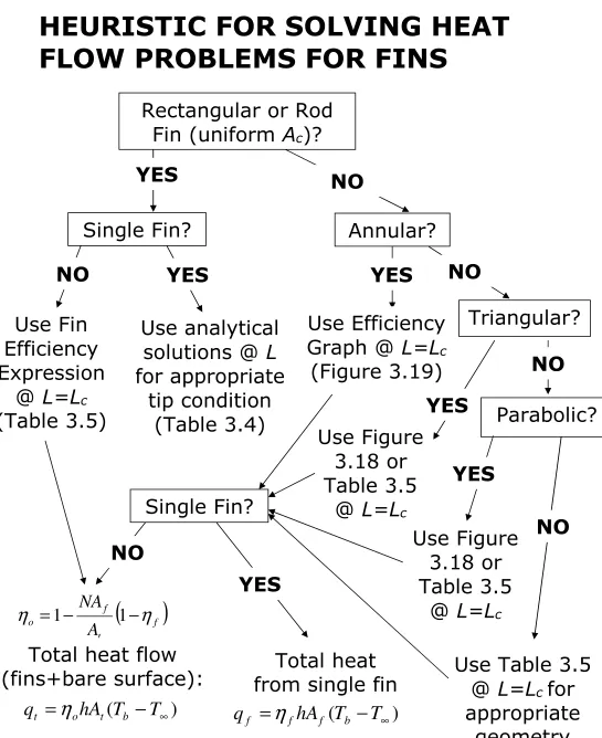
HEURISTIC FOR SOLVING HEAT FLOW PROBLEMS FOR FINS

Single Fin? Use analytical

solutions @ L

for appropriate tip condition

(Table 3.4)

YES _NO

Annular? Rectangular or Rod

Fin (uniform Ac)?

YES

Use Fin Efficiency Expression

[image:81.612.37.582.64.732.2]

@ L=Lc

(Table 3.5)

YES NO

Use Efficiency Graph @ L=Lc

(Figure 3.19)

Triangular?

YES

NO

Use Figure 3.18 or Table 3.5

@ L=Lc

Parabolic?

YES

NO

Use Figure 3.18 or Table 3.5

@ L=Lc

Use Table 3.5 @ L=Lc for

appropriate geometry Single Fin?

NO

YES NO

) ( − _∞

= hA T T

q_f η_{f f b}

Total heat from single fin

(

f

)

t f o

A NA

η η =1− 1−

) ( − _∞

= hA T T

q_t η_{o t b}

Total heat flow (fins+bare surface):