Recommender systems with Bayesian aspect models and the effect of approximate inference

(1)

by

Dylan Verrezen

Thesis presented in partial fulfilment of the requirements

for the degree of Master of Science in Engineering in the

Faculty of Engineering at Stellenbosch University

Supervisor: Prof. J.A. du Preez

(2)

Abstract

Recommender Systems with Bayesian Aspect Models

and the Effect of Approximate Inference

D. Verrezen

Department of Electrical Engineering, University of Stellenbosch, Private Bag X1, Matieland, 7602.

Thesis: MScEng

March 2018

Recommender systems form an important part of the modern world. These systems allow users to find relevant items in often huge item collections. Col-laborative filtering is a pervasive and popular form of recommender that rec-ommends to users based on their histories and the histories of other users. The field was long dominated by two forms of collaborative filtering: neigh-bourhood methods and matrix factorisation models. The two approaches were based on the assumption that the better the prediction of the rating a user would give an item, the greater the quality of the recommendations. This assumption has been criticised as being misleading. One major criticism is that the recommender systems are not being evaluated on the quality of the actual recommendation list. The systems are instead being evaluated on how well they perform a proxy task: predicting ratings. Another criticism is that it leads to recommenders that overfit to popular items that have the majority of the observed feedback. One possible improvement is to instead evaluate recommender systems by how effectively they rank items by determining how many relevant items they can return for a user in their top N results. However,

(3)

traditional, popular forms of collaborative filtering perform these tasks poorly. To address this we turn to Bayesian aspect models. These models come from the field of topic modelling. These aspect models are unsupervised models that express co-occurrence data in terms of latent aspects, where aspects are collec-tions of thematically related items. The best known and most powerful aspect model is Latent Dirichlet Allocation, and preliminary literature suggests that it performs very well for recommendation tasks. A drawback to these Bayesian aspect models is that exact inference is intractable and we need to turn to ap-proximate inference techniques. In this document we verify the performance of Latent Dirichlet Allocation for recommendation, and investigate the effect of approximate performance on the results for recommendation tasks.

(4)

Uittreksel

Recommender Systems with Bayesian Aspect Models

and the Effect of Approximate Inference

D. Verrezen

Department of Electrical Engineering, University of Stellenbosch, Private Bag X1, Matieland, 7602.

Tesis: MScEng

Maart 2018

Aanbevelingstelsels speel ’n belangrike rol in die moderne wêreld. Hierdie stel-sels stel gebruikers in staat om relevante items op te spoor in (dikwels) groot versamelings data wat oor verskeie domeine kan strek. Samewerkende filtre-ring maak gebruik van die soortgelykhede tussen ’n gebruiker se geskiedenis en dié van ander gebruikers om aanbevelings te maak. Hierdie veld was lank gedomineer deur twee vorme van samewerkende filters: buurtmodelle en ma-triksfaktorisering. Die twee benaderings was gegrond op die veronderstelling dat ’n beter voorspelling van die telling wat ’n gebruiker aan ’n item sou gee, noodwendig ook sal lei tot hoër gehalte aanbevelings. Hierdie aanname blyk misleidend te wees – die tellings wat ’n gebruiker gee is nie direk ekwivalent aan die nuttigheid van ’n aanbeveling nie. Verder lei dit ook tot ’n oormatige fokus op populêre items wat volop in die beskikbare data voorkom. Gevolglik het die veld verskuif na nuwe vorme van evaluering. ’n Moontlike benadering is om eerder aanbevelingstelsels te baseer op hoeveel van die items in die boonste N aanbevelings relevant vir die gebruiker was. Die tradisionele gewilde vorme van samewerkende filtrering vaar nie juis goed met hierdie tipe evaluering nie. Om

(5)

meer toepaslike stelsels te ontwikkel, wend ons ons tot Bayesiese aspekmodelle. Hierdie modelle is gewild in die veld van onderwerpsmodellering. Hierdie tipe van modelle kan sonder eksplisiete toesig assosiasies maak tussen items wat dikwels saam in tematies-verwante data voorkom. Die bekendste en sterkste aspekmodel is die sogenaamde latente Dirichlet-toekenningtegniek. Voorlo-pige ondersoeke dui daarop dat dit belofte vir aanbevelingstake mag inhou. ’n Nadeel van hierdie Bayesiese modelle is dat presiese inferensie wiskundig onhaalbaar is – dit noop mens om dit met benaderingstegnieke te takel. In hierdie dokument verifieer ons die nuttigheid van latente Dirichlet-toekenning vir aanbeveling, en ons ondersoek ook die rol wat benaderingstegnieke ten opsigte van aanbevelingstake speel.

(6)

Declaration

By submitting this thesis electronically, I declare that the entirety of the work contained therein is my own, original work, that I am the sole author thereof (save to the extent explicitly otherwise stated), that reproduction and pub-lication thereof by Stellenbosch University will not infringe any third party rights and that I have not previously in its entirety or in part submitted it for obtaining any qualification.

March 2018

Date: . . . .

(7)

List of Figures

2.1 Applying Bayes’ rule to estimate a coin’s bias . . . 20

2.2 Bayes network when determining coin bias . . . 24

2.3 Example Bayes network with five random variables . . . 25

2.4 The three possible inactive triplet Bayes network configurations . 27 2.5 The three possible active triplet Bayes network configurations . . 27

2.6 Bayes net for determining coin bias fromN flips . . . 29

2.7 Three Normal(Gaussian) distributions visualised together . . . 31

2.8 Two different binomial distributions . . . 32

2.9 A uniform Dirichlet distribution . . . 35

2.10 A concentrated Dirichlet . . . 35

2.11 A sparse Dirichlet . . . 36

3.1 A simple example of a feedback matrix . . . 41

3.2 Confusion Matrix . . . 44

3.3 Matrix factorisation based recommendation. . . 51

3.4 Graphical model for asymmetric PLSA. . . 58

4.1 Latent Dirichlet Allocation Bayes Network . . . 64

4.2 Topic distribution word clouds . . . 68

4.3 Movie Aspects from an LDA recommender . . . 71

5.1 Minimising KL (q||p) for multimodal distributions . . . 87

5.2 Minimising KL (p||q) for multimodal distributions . . . 88

5.3 Mean field approximations . . . 93

5.4 Aspect distributions from LDA inference with EP on an artificial dataset . . . 106

(14)

5.5 Aspect distributions from LDA inference with VI on an artificial

dataset . . . 107

5.6 Aspect distributions from LDA inference with VI on an artificial dataset. The LDA was trained with 4 aspects when the artificial dataset is known to have 10. . . 108

5.7 Aspect distributions from LDA inference with EP on an artificial dataset. The LDA was trained with 4 aspects when the artificial dataset is known to have 10. . . 109

5.8 Aspect distributions from LDA inference with VI on an artificial dataset. The LDA was trained with 10 aspects when the artificial dataset is known to have 10. However the user mixture prior was set sparse when the true distribution is dense. . . 110

5.9 Aspect distributions from LDA inference with EP on an artificial dataset. The LDA was trained with 4 aspects when the artificial dataset is known to have 10. However the user mixture prior was set sparse when the true distribution is dense. . . 111

6.2 Experiment 1: F1 score comparison of inference methods . . . 120

6.3 Experiment 2: Recall results . . . 122

6.4 Experiment 2: Precision results . . . 123

(15)

List of Algorithms

1 Metropolis-Hastings algorithm . . . 81 2 Gibbs Sampling . . . 82 3 Gibbs sampling example for a model with three parameters . . 82 4 Collapsed Gibbs sampling example for a model with three

pa-rameters with one collapsed out . . . 83 5 Collapsed Gibbs inference procedure for Latent Dirichlet

Allo-cation . . . 86 6 Coordinate Ascent Mean Field Variation Inference . . . 94 7 Variational parameter update procedure for user level

parame-ters when performing inference for Latent Dirichlet Allocation 97 8 Full Variational EM procedure for Latent Dirichlet Allocation 98 9 General Expectation Propagation . . . 101

(16)

Nomenclature

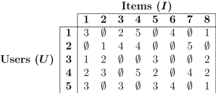
General Recommendation R Feedback Matrix U Number of users I Number of items u A single user i A single item

ru,i Explicit feedback user ugave item i yu,i Implicit feedback useru gave item i

ˆ

ru,i Predicted feedback user u gave itemi

µ Mean

σ Standard deviation

Matrix factorisation K Number of features

V User feature matrix for all users

Y Item feature matrix for all items ˆ

R Predicted feedback matrix

Latent Dirichlet Allocation K Number of aspects

z Aspect membership indicator

β Aspect-item distribution. A K×I random matrix

βk Item distribution for aspect k xv

(17)

η I-dimensional Dirichlet parameter for the prior on βk

θu Useru’s aspect mixture. A K dimensional multinomial

α K-dimensional Dirichlet parameter for the prior on θu Approximate Inference

x(t) _{The state of the random variable}_x _{at time}_t π The stationary distribution of a Markov chain

Q A proposal distribution

x−i All of the elements in the vector x, except the i-th element Gibbs Sampling for Latent Dirichlet Allocation

N−n,k Number of items assigned to aspect k excluding the current item Ni

−n,k Number of times item ihas been assigned to aspect k excluding the

current item

Nu

−n,k Number of items assigned to aspectkfor useruexcluding the current

item

N₋u_n Number of items observed for user uexcluding the current item

Variational Inference for Latent Dirichlet Allocation

λk Variational Dirichlet parameter on the variational approximation to

βk

γu Variational Dirichlet parameter on the variational approximation to

γu

φu,n Variational Multinomial parameter on the variational approximation

tozu,n

Mathematics

exp(x) The natural exponent of x, (ex₎

IN The identity matrix. A matrix with 1 for all diagonal values and 0

otherwise with rankN 1 A vector of all ones

(18)

KL (p||q) Kullback-Leibler divergence betweenp and q

Distributions

Dir(α) Dirichlet with parameter α

Multi(p) Multinomial with probabilities p

Abbreviations

RV Random Variable

PDF Probability Density Function PMF Probability Mass Function

CDF Cumulative Distribution Function MLE Maximum Likelihood Estimation MAP Maximum a Posteriori

SVD Singular Value Decomposition

PLSA Probabilistic Latent Semantic Analysis LDA Latent Dirichlet Allocation

GAM Generative Aspect Model MCMC Markov Chain Monte Carlo KL Kullback-Leibler

VI Variational Inference ELBO Evidence Lower Bound

CAVI Co-ordinate Ascent Variational Inference SVI Stochastic Variational Inference

ADVI Automatic Differentiation Variational Inference ADF Assumed Density Filtering

EP Expectation Propagation LBP Loopy Belief Propagation

(19)

Chapter 1 Introduction

1.1 Motivation

Recommender systems are an important part of modern life. The sheer volume of content exposed by the internet requires systems that enable users to filter out relevant items from huge online collections. The basic task of a recom-mender system is to generate a list of relevant items for a user. This list could be movies that a user will enjoy, or items that a user would purchase. Recom-mender systems form an important part of many commercial systems such as for recommending video media at Netflix (Gomez-Uribe & Hunt, 2015), items for purchase at Amazon (Linden et al., 2003; Smith & Linden, 2017) or news articles for the New York Times (Spangher, 2015). Recommender systems have also been used for other diverse tasks such as helping researchers find scientific articles (Wang & Blei, 2011).

1.2 Background

Originating in the mid-90s, the earliest recommender systems were based on collaborative filtering (Resnick et al., 1994; Shardanand & Maes, 1995; Hill

et al., 1995), where the recommendation was based on the behaviour of sim-ilar users. The dominant method for evaluating recommender systems was based on predicting the rating a user would give an item. These early systems were based on neighbourhood methods. Neighbourhood methods generated

(20)

recommendations for a user by finding a neighbourhood for a user that con-sisted of similar users. The recommender system could then predict the ratings based on the ratings that similar users gave items. These methods are known as memory-based recommenders, because they do not construct any explicit model (Ekstrand et al., 2011). These approaches remain a core approach for recommendation today, as they are intuitive and simple to implement (Schafer

et al., 2007).

1.2.1 Ratings Prediction Systems

These early methods generated recommendations by first predicting the rating a user would give an item. Items could then be recommended based on the predicted rating. These predictions were evaluated with average error metrics such as Root Mean Square Error (RMSE) between the predicted and actual ratings. With ratings, users directly indicate their preference; such ratings data is known as explicit feedback. The choice to focus on evaluating recom-mender systems with explicit data was in part driven by the fact that explicit data was the only form of feedback available (Gomez-Uribe& Hunt, 2015). By considering explicit feedback as a measure of user preference, the assumption was that improving the accuracy would provide better recommendations.

The focus on ratings prediction culminated in the Netflix Prize competition. The Netflix Prize was a competition with a $1,000,000 prize that would be awarded to the team that could achieve a 10% improvement over Netflix’s own recommender system (Bell & Koren, 2007). The task was ratings prediction and was measured via RMSE. The Netflix Prize led to the development and subsequent popularity of matrix factorisation models. These models are closely related to dimensionality-reduction techniques such as Principal Component Analysis and low-rank singular value decomposition approximations. The core idea behind matrix factorisation models is to map users and items to a common low-rank feature space. The low rank of the feature space acts to bottleneck the model so that it can find general features that describe the users and items. Rating prediction can be performed using the feature representations of the users and items (Koren et al., 2009).

(21)

1.2.2 Matrix Factorisation Models

The first matrix factorisation models used singular value decomposition (SVD) to find the feature representations of users and items. The SVD-based ma-trix factorisation model is commonly referred to as PureSVD to differentiate from models that came after (Koren et al., 2009). A problem for PureSVD is that recommendation datasets are extremely sparse, i.e. most of the user-item feedbacks are unobserved. The singular value decomposition is not defined for sparse datasets and the workarounds to this are computationally expensive. A breakthrough for matrix factorisation models came in the form of an approxi-mate method of calculating the SVD just using the observed data. The method uses stochastic gradient descent to learn the user and item features directly. The approximate SVD model led to increased interest in matrix factorisation models after it jumped to third place on the Netflix Prize leaderboards (Funk, 2006). This was despite its relative simplicity compared to the complex en-sembles of models being used at the time.

Team Bellkor was a very successful team over the course of the Netflix com-petition and made heavy use of matrix factorisation models. They developed two extensions to the SVD based approaches, namely Asymmetric-SVD and SVD++ (Bell et al., 2008). Team Bellkor ultimately won the Netflix Prize after joining up with another team, and the winning approach made heavy use of matrix factorisation models.

While the competition was a success and spurred the development of many new approaches to recommendation, the winning solutions involved complex ensembles of models that were impractical for real-world use (Gomez-Uribe &

Hunt, 2015). However, Asymmetric-SVD and SVD++ remain state of the art for rating prediction, and matrix factorisation models became a core approach to recommendation.

1.2.3 Topic Models

Matrix factorisation models are not limited to recommender systems: early topic models also used matrix factorisation techniques. Topic modelling is a

(22)

field of information retrieval that attempts to find the latent semantic struc-ture for collections of text (Blei & Lafferty, 2009). Topic models describe documents in terms of latent topics and aim to enable the indexing and dis-covery of documents in large document corpora. An early topic model was Latent Semantic Analysis (LSA), which used a low-rank SVD approximation to map documents to the topic space, much in the same way as PureSVD would for recommendation. Hofmann (1999) gives an equivalent statistical model to LSA in the form of Probabilistic Latent Semantic Analysis (PLSA). PLSA attempted to improve over LSA by finding better topics and to provide a statistical backing to explain why the matrix factorisation approach works.

PLSA tended to overfit and to address this Blei et al. (2003) extended PLSA to a Bayesian statistical model known as Latent Dirichlet Allocation (LDA). Latent Dirichlet Allocation has been very successful for topic modelling (Blei, 2012) and has been applied to many collections of documents, including news-paper articles (Wei & Croft, 2006) and scientific abstracts (Blei et al., 2003). Whereas topic models have been suggested for recommendation, they are ill-suited to rating prediction and failed to make much of an impact. When used for recommendation, topic models bypass predicting the ratings and instead directly predict items for a user. Hofmann (2004) develops PLSA for collabora-tive filtering and devises extensions to the model to enable ratings prediction. Blei et al.(2003) also suggests that LDA could be used for collaborative filter-ing.

1.2.4 Ratings Prediction versus Top-N

Recommendation

The reason topic models cannot natively perform ratings prediction is that they were originally designed to work with word counts in documents. Recommen-dation also has a form of count data in the form of implicit feedback. Implicit feedback consists of observations of user behaviour that indirectly indicates user preference. This could be counts of how many times a user viewed an item or clicked a link. With the exploding popularity of the web, the amount

(23)

of implicit data saw a sharp increase. For example at Netflix their early focus on ratings data was based on the fact that when they were mailing DVDs to people, ratings were the only form of feedback they received (Gomez-Uribe &

Hunt, 2015).

The need to work with implicit data and criticisms of ratings prediction as an evaluation method has led to alternative methods of evaluating recom-mender systems. Ratings prediction has been criticised because it measures recommendation performance based on the predicted rating and not on the quality of the recommendation list (Cremonesiet al., 2010). Another criticism is that the focus on predicting the rating leads to models that overfit on pop-ular items in the dataset (McNee et al., 2006). Additionally, in practice the assumption that better ratings prediction led to higher quality recommenda-tions was misleading (Gomez-Uribe & Hunt, 2015). An alternative method of evaluating recommender systems is instead to evaluate the accuracy of the recommendation list produced. One such method is to evaluate systems based on how many relevant items they can produce for a user in the system’s top-N

predictions.

Many of the state-of-the-art systems for recommendation perform poorly when evaluated via top-N prediction. Cremonesi et al. (2010) showed that simple early core approaches such as neighbourhood models and PureSVD matched and even exceeded the performance of state-of-the-art systems such as Asymmetric-SVD and Asymmetric-SVD++. When performing evaluation via top-N prediction, the LDA model’s inability to predict ratings is no longer a problem. Other evalua-tions of recommenders suggested that probabilistic approaches perform well for item prediction (Barbieri & Manco, 2011). With the shifting focus towards item prediction, we can revisit topic models like LDA for recommendation. This document aims to develop the LDA model in the context of recommen-dation and to show how it evolved from matrix factorisation models. It also aims to evaluate how LDA performs for item prediction compared to the core recommender system methods. One specific case of recommendation that is of particular interest is recommending to new users in a system. This is a chal-lenging task, because a new user has little or no history from which to generate

(24)

recommendations. This is known as the cold-start problem. Bayesian models are known to gain accuracy quickly using little data (Ng & Jordan, 2002). Investigating how LDA works in a cold-start scenario is therefore of particular interest.

1.2.5 Bayesian Models and Approximate Inference

A drawback of Bayesian models is that for many interesting models includ-ing LDA, exact inference is intractable. When performinclud-ing Bayesian inference we are interested in calculating the posterior distribution of the model. The posterior is the distribution of the model’s variables given the observed data. Unfortunately, calculating the posterior involves integrals that are intractable.

This means we must turn to approximate inference algorithms to learn the model parameters. A popular approach to approximate inference is Markov Chain Monte Carlo (MCMC) methods. These methods leverage Monte Carlo integration and samples from a Markov chain to approximate the intractable integrals involved in inference (Gilks et al., 1995). Other approaches involve finding a simpler approximate posterior that is close to the true posterior. Methods that do so rely on minimising some divergence measure between the approximate and true posterior. One such divergence measure is Kullback-Leibler divergence. Kullback-Kullback-Leibler divergence is not symmetrical, meaning that for a posterior p and approximate posteriorq the Kullback-Leibler diver-gence between p||qis not the same as that betweenq||p. Two approaches that find approximate posteriors by minimising the Kullback-Leibler are Variational Inference (VI) (Blei et al., 2017) and Expectation Propagation (EP) (Minka, 2001). VI and EP use the opposing symmetries of the Kullback-Leibler diver-gence as each other to find the approximate posterior. What is not clear is the effect that the assumptions, simplifications and objectives of these approxi-mate inference algorithms will have on the LDA performance in practice. This document also seeks to investigate how the choice of approximate inference will affect the suitability of the LDA model for recommendation.

(25)

1.3 Goals

1. Develop a recommender system based on LDA.

2. Compare recommenders based on LDA against the core recommendation approaches.

3. Investigate the effect that approximate inference has on recommendation accuracy when using LDA for recommendation.

4. Investigate LDA for cold-start recommendation.

1.4 Contributions

1. Re-formulating a number of recommendation systems in a common frame-work, thereby making their interrelationships clear.

2. C++ code implementations of the following approximate inference algo-rithms for LDA:

a) Variational inference. b) Collapsed Gibbs sampling. c) Expectation Propagation.

3. Python code implementations of the following recommendation approaches: a) Neighbourhood methods.

b) The matrix factorisation model: PureSVD.

4. Experimental results performed on a dataset of one million ratings from the MovieLens data set:

a) Showing that the LDA recommender consistently outperforms tra-ditional approaches for top-N recommendation.

b) Showing that the LDA recommender gains its advantage from im-proved personalisation.

c) Showing that the LDA recommender has promising results for cold-start recommendation.

(26)

1.5 Overview

We are interested in evaluating the LDA topic model for recommendation. LDA is a Bayesian generative model. Bayesian statistics consider probability as a rational measure of uncertainty and treat all uncertain variables, includ-ing the model parameters, as random variables. Chapter 2 provides a review of some theoretical background for the Bayesian model. An important part of this is covering how the models are represented as a generative process (Section 2.1.3) coupled with a graphical model (Section 2.7). The graphical model rep-resentation helps to illustrate the dependency structure of the model (Section 2.7). This allows us to factorise the model’s joint distribution into a product of conditional distributions for the model parameters. This representation is also useful as many of the inference techniques in Chapter 5 require a factorised representation of the model.

Before developing LDA for recommendation, we cover it precursor models. Many state-of-the-art collaborative filtering recommender systems are based on matrix factorisation.

1.5.1 Recommender Systems

Recommender systems are tasked with discovering new items for users that they will enjoy. A common representation for recommender systems is the feedback matrix: RU×I =        r1,1 r1,2 · · · r1,I r2,1 r2,2 · · · r2,I .. . ... . .. ... rU,1 rU,2 · · · rU,I        . (1.1)

The feedback matrix is a matrix of all the implicit or explicit feedback ob-served from users, placed into spares matrices with users as rows and items in columns. Many early recommender systems were evaluated on how well they could predict the missing values of the matrix. More recently, evaluation of recommender systems has started instead to move towards evaluating the

(27)

sys-tem on how well it can predict the isys-tems a user would choose. More detailed coverage of the recommendation problem is given in Section 3.1.

Recommendation accuracy is not the only factor when evaluating recommender systems. There are many other important aspects that should be considered when designing or evaluating a recommender. One of the most important is

explainability, whereby the recommendations provided by the system can be explained to the user. Users generally prefer recommendations where they understand why items are being recommended to them. Matrix factorisation methods often cannot generate explainable recommendations.

Matrix factorisation methods for recommendation are covered in Section 3.5. The core idea of these methods is to map users and items to a latent feature space that is of a lower dimension that the feedback matrix. To do so, the simplest methods factorise the feedback matrix into lower-ranked feature ma-trices, namely a user- and an item-feature matrix. Ratings can be predicted by the dot product of a user and item in feature space. Recommendations are then performed by ranking items by their predicted ratings.

Probabilistic Latent Semantic Analysis (PLSA) is a statistical interpretation of matrix factorisation models. PLSA restricts the feature space to be a valid probability distribution. In doing so, items are characterised by their member-ship to aspects. An aspect is a distribution over all the items and captures the notion of a user community, or items that frequently occur together for certain users. The users are characterised by their membership of aspects and they can proportionally belong to several aspects. This characterisation captures how users belong to the pseudo-communities or how they can have diverse interests. PLSA suffered from drawbacks such as overfitting, much like matrix factorisation models, and it did not capture all the available relationships be-tween items.

LDA further extends PLSA to be fully Bayesian. This addresses some of the overfitting concerns and allows for the use of the tools from Bayesian modelling, such as easy model extensions. In theory LDA is a good model for

(28)

recommendations - it directly estimates the probability of users choosing items and it naturally partitions users into communities and items into clusters. It is a standard model for topic modelling; however, it is not well understood for recommendation.

1.5.2 Approximate Inference

A hurdle to working with Bayesian models is that all models must define a valid joint probability distribution over the observed data and the model pa-rameters. For most interesting models this involves intractable integrals. We can instead turn to approximate methods that estimate the posterior distri-bution of the model.

One possible approach to approximate inference is to use sampling methods as shown in Section 5.2. Markov Chain Monte Carlo (MCMC) is a sampling method that constructs a Markov chain to draw samples from the posterior distribution of the model. It then uses Monte Carlo integration with the gen-erated samples to approximate the intractable integrals with sums.

The second class of approximate inference method reframes inference as an optimisation problem. By defining an approximate posterior, the goal be-comes to optimise the approximation to be as close as possible to the true posterior. To do so, such methods minimise a divergence measure between the approximate and true posterior. A common divergence measure used for this is Kullback-Leibler divergence; however, Kullback-Leibler divergence is not symmetrical. The choice of whether to minimise between the true and ap-proximate or vice-versa changes the nature of the apap-proximate posterior found. More discussion on Kullback-Leibler divergence can be found in Section 5.3.

Variational Inference and Expectation Propagation are two such approaches that minimise Kullback-Leibler divergence. Both approaches will approximate a multi-modal distribution with a simpler distribution with some key differ-ence. Variational Inference is mode-seeking, and will find an approximate distribution that closely matches one of the true distribution’s modes. In

(29)

contrast, Expectation Propagation is moment-matching, and will find an ap-proximate distribution that averages over the modes of the true distribution. The found approximation has moments that match the moments of the true distribution. Variation Inference is discussed in Section 5.4 and Expectation Propagation in secion 5.5.

1.5.3 Key Results and Conclusions

The goal of the experiments was to investigate how well LDA performs for recommendation in comparison to the core recommender approaches, and to evaluate how much the choice of approximate inference technique affects the performance of LDA. Our first experiment compared Latent Dirichlet Alloca-tion to the best-performing approaches from Cremonesi et al. (2010). LDA utilising variational inference consistently outperformed the other approaches. The effect of inference was noticeable and the LDA had similar performance to the other approaches when not using variational inference.

The second experiment dug deeper into LDA’s strong results in an attempt to uncover whether the accuracy arose from improved personalisation of the rec-ommendations. To investigate the effect of personalisation, recommendations were made from the same trained LDA model via two methods. The first was the standard personalised approach, while the second ignored the user features and generated recommendations directly from the global item features. When unpersonalised, the LDA model performs similarly to the other recommenda-tion methods. This indicates that most of the improvement came from better tailoring the recommendations to the users and not from finding better general recommendations.

The final experiment explored LDA in cold-start scenarios. A cold start in recommendation is when the system has to recommend to users with little or no history, e.g. new users. For this experiment only a small fraction of the test set user ratings were used for training. The LDA still performed well, but not drastically better as it did in the regular case.

(30)

Overall Latent Dirichlet Allocation showed very promising performance when used for recommendation. The effect of approximate inference cannot be ig-nored, however. Variational inference made the difference between LDA per-forming roughly as well as the other approaches, or perper-forming nearly twice as well. A further advantage for LDA is that it is a popular and well-studied model for topic modelling. Many extensions that may improve the model for recommendation already exist. Further investigation of LDA for tion could consider how these existing extensions could enable recommenda-tion. Alternatively, LDA’s Bayesian nature allows for it to be easily adapted to new recommender domains or to find novel extensions specifically for rec-ommendation.

(31)

Chapter 2 Bayesian Modelling

Statistical modelling forms an important part of the scientific process and for machine learning. We will cover the model Latent Dirichlet Allocation, which is a Bayesian model over co-occurrence data. This chapter gives some brief theoretical background on Bayesian modelling and how the models are represented; Latent Dirichlet Allocation is covered in the next chapter.

2.1 Statistical Modelling

Statistical modelling is concerned with modelling some data-generating pro-cess where some or all of the variables involved are stochastic. When a variable is stochastic we refer to it as a random variable (RV). A random variable is the numerical outcome of a random process and does not have a fixed determinis-tic value, but we instead describe it via a probability distribution (Peebles &

Shi, 2001). The probability distribution assigns a probability (or a probability density in the case of continuous RVs) to every possible value of the random variable. Probability itself is generally interpreted in one of two ways: frequen-tist or Bayesian (Bishop, 2006). The two different perspectives on probability lead to different approaches in modelling.

2.1.1 Frequentist and Bayesian Paradigms

The frequentist or classical viewpoint denotes probability as the relative fre-quency of a random and repeatable event. Frequentist modelling regards the

(32)

observed data as random and unreliable and seeks to estimate the true value of the model parameters (Bishop, 2006).

By contrast, the Bayesian viewpoint is a more general view of statistics that considers probability as a rational, conditional measure of belief (Bishop, 2006). The Bayesian paradigm is axiomatic and all methods only require the interpretation of probability as a measure of uncertainty and the mathematics of probability theory. It has been shown that in terms of the Bayesian view-point, probability theory is an extension of Boolean logic with uncertainty (Jaynes, 2003). A central component of this approach is that all unknown quantities are described by probability distributions. This includes the model parameters. The probability distributions over the variables quantify our un-certainty about the variables and allow us to revise these beliefs with new evidence. A characteristic of the Bayesian approach is thatprior distributions must be supplied that describe the initial beliefs about variables and param-eters. This allows for prior knowledge to be naturally included in models (Bishop, 2006).

2.1.2 Generative Models

Statistical models specify a model that is assumed to describe the true process generating the observable data, hence the name generative models. A char-acteristic of generative models is that they can be sampled to produce syn-thetic data. Modelling involves many simplifying assumptions and the true distribution of the data is probably far too complex to precisely capture, but models can still serve as useful approximations to reality (Burnham & An-derson, 2003). Recommender systems typically have extremely sparse input observations, and generative models have been shown to work well with few observations (Ng & Jordan, 2002).

2.1.3 Generative Process

To specify a generative model, we can specify a pseudo-code-style process that specifies how each variable is generated. For a simple model with a single

(33)

distribution over the vector observations x parametrised by a parameter ζ, the basic generative process would be:

1. Sample the model parameters from the prior ζ ∼p(ζ).

2. Select (sample) each observationx inxfrom the data-generating distri-bution: x∼p(x|ζ).

2.2 The Rules of Probability

Bayesian statistics uses the mathematics of probability theory to represent uncertainty. The two most important rules of probability for Bayesian methods are the sum and the product rule.

2.2.1 The Sum Rule

For two discrete RVs x and y with a joint discrete probability distribution p(x, y), the sum rule allows us to get the marginal probability mass function of x:

p(x) =X

y

p(x, y). (2.1)

Equivalently, if x and y are continuous, the marginal probability density of x

is found by integrating out y:

p(x) =

Z

p(x, y)dy. (2.2)

2.2.2 The Product Rule

The second rule is the product rule. The product rule gives the relationship between the joint distribution and the conditional probability, p(y|x):

p(x, y) = p(y|x) p(x) = p(x|y) p(y). (2.3)

Using the symmetry property for the joint distribution

(34)

and by applying the product rule twice, we can obtain the inverse probability

2.3 Bayesian Models

Consider the general case where we have observed some data D and we wish to learn something about the process that generated the observations. To do so we construct a generative model with parameters ζ over the variables we have measured. Under the Bayesian paradigm the observations and model parametersζ are considered as random variables and the model defines a joint distribution over them p(D,ζ). The key problem is then finding an appropriate choice of model parameters, or using the Bayesian perspective quantify the uncertainty about their values. Specifically we are interested in the probability distribution over the model parameters given the observed data. This is known as the posterior probability:

posterior = p(ζ | D). (2.6) The posterior probability can be represented explicitly using Bayes’ theorem (equation 2.5) in the form (Bernardo, 2003):

p(ζ | D) = p(D | ζ) p(ζ)

p(D) . (2.7)

This requires first specifying a prior distribution p(ζ) over the model param-eters, capturing the assumptions or the initial beliefs about the parameters. The data affects the posterior through its influence in the likelihood function p(D |ζ) in the numerator. The likelihood function is a function of the model parameters and evaluates how probable the observations are for the different values that the parameters could take. The likelihood function is not a valid probability distribution and does not necessarily integrate to one (Bishop,

(35)

2006).

The denominator p(D) is known as the evidence or marginal likelihood. It ensures that the posterior distribution is a valid distribution that integrates to unity (or sums if the posterior is discrete).

p(D) =X ζ p(D |ζ) p(ζ) or p(D) = Z p(D |ζ) p(ζ)dζ. (2.8)

The marginal likelihood is often omitted to give Bayes’ rule in proportional form:

posterior∝likelihood×prior p(ζ | D)∝p(D |ζ) p(ζ).

(2.9)

The Bayesian approach is inherently iterative, and as new observations come in, the previous posterior can be used as a prior (both are distributions over the model parameters) in Bayes’ rule to get an updated posterior with the new data. The model can update its beliefs (the posterior) as evidence comes in while taking into account its current beliefs (the prior).

2.3.1 Hierarchical Models

For models that do not just consist of a single distribution for the likelihood and prior, a more efficient representation is needed. In hierarchical models the statistical model is represented as a series of sub-models (Allenbyet al., 2005). Essentially the model consists of multiple levels of priors (Rouderet al., 2013). A simple two-stage hierarchical model which has a likelihood:

p(x|ζ) (2.10)

a prior on ζ with hyperparameter φ:

(36)

and the hyperprior on φ:

p(φ) (2.12)

combining to get the posterior:

p(ζ, φ|x)∝p(x|ζ) p(ζ |φ) p(φ) (2.13)

2.3.2 Conditionally Conjugate Models

The specific class of hierarchical Bayesian models that Latent Dirichlet Al-location belongs to are conditionally conjugate models. These models have levels of variables, split into local and global levels. Typically each observa-tion is accompanied by a local latent variable. The global variables control the distribution over the latent variables.

2.4 Applying Bayes’ Rule

To illustrate how Bayes’ rule updates beliefs, we consider the simple example of trying to determine if a fair looking coin is biased. In the extreme case, if the coin is flipped a few times and comes up the same tails each time, the maximum likelihood estimate will suppose that the tails has a probability of 1, implying that all future flips will come up tails. With an appropriately chosen prior, the Bayesian approach can help avoid this overfitting but at the cost of having to choose a sensible prior distribution.

To do so, we consider a simple model with the bias of a coin θ as the proba-bility it comes up heads. A normal fair coin will have a bias of θ = 0.5 where heads and tails are equally likely, but we consider the case where we suspect the coin is biased toward one face, perhaps to give an edge in a game of chance.

The generative process for the biased coin example is given:

1. Select a bias by sampling from a symmetrical Beta distribution: θ ∼

Beta(α, β) with equal parameters α=β

2. For each coin toss, the result xn is chosen as heads with probability θ

(37)

We represent our prior beliefs about the coin as a symmetrical Beta distribu-tion with equal hyperparameters so that it is centred on 0.5. The PDF for the Beta distribution is given in equation 2.14 where the function B(α, β) is a normalising function.

p(θ |α, β) = θ

α−1₍₁₋_θ₎β−1

B(α, β) (2.14) If we flip the coin N times and observe k heads, our likelihood is given by the Binomial PMF where N_k is the Binomial coefficient:

p(k |θ, N) = N k θk(1−θ)N−k. (2.15) We can now use Bayes’ rule to update our belief about the bias θ with the observed k heads from N flips:

p(θ |k, α, β)∝ N k θk(1−θ)N−kθ α−1₍₁₋_θ₎β−1 B(α, β) (2.16) Folding all normalising functions and constants into the implied normaliser in Bayes rule we get:

p(θ |k, α, β, N)∝θk(1−θ)N−kθα−1(1−θ)β−1 p(θ |k, α, β, N)∝θα+k−1(1−θ)β+N−k−1

(2.17)

Which, when we consider the form of the Beta distribution in equation 2.14 is a Beta distribution with parameters α+k and β+N −k.

p(θ|k, α, β, N) = Beta (α+k, β+N −k). (2.18) In figure 2.1 the prior is shown with the posterior. We can see that after observing 8 heads out of 10 flips, the model believes that the coin may be biased. The belief is not extreme, however, as the data needs to overcome the prior. The prior in essence acts to regularise the model and allows us to represent our previous knowledge about it.

2.4.1 Maximum Likelihood and Maximum a Posteriori

Estimation

In contrast to the Bayesian approach, the frequentist viewpoint considers the data to be uncertain or incomplete and wishes to estimate the fixed value

(38)

Figure 2.1: The prior Beta distribution (shown in blue) and the updated pos-terior distribution (shown in green) that we obtain after observing eight heads from ten coin flips. The two distributions are shown together to illustrate how the posterior represents our uncertainty about the coin. With the relatively low number of flips our updated belief suggests that the coin may be slightly biased but does not assume that the coin has a bias of 0.8 as a naive estimate would assume.

of the model parameters ζ. The uncertainty of this estimate can be shown with error bars obtained by considering the distribution of possible datasets (Bishop, 2006).

One possible method of obtaining estimates of the model parameters is via maximum likelihood estimation (MLE). MLE chooses the values for ζ that best explain the observed data by finding the values for ζ that maximise the likelihood:

ˆ

ζM LE = arg max ζ

(39)

Another method for obtaining a fixed-point estimate of the parameters that incorporates a prior is via Maximum a Posteriori (MAP) estimation. MAP finds settings for the parameter values by maximising the posterior as opposed to the likelihood. By exploiting the fact that the marginal likelihood does not depend on ζ and is always positive, we can drop the denominator from Bayes’ rule and get the MAP estimator as:

ˆ ζM AP = arg max ζ p(ζ | D) = arg max ζ p(D |ζ) p(ζ). (2.20) These approaches differ from the Bayesian perspective where ζ is not consid-ered as a fixed parameter but instead the uncertainty about ζ is expressed for the given data in the posterior. A disadvantage to the Bayesian approach is that it requires calculating the marginal likelihood - the integral of which can, and often will for interesting models, become intractable to compute. In these cases we must turn to methods that approximate the posterior.

2.5 Choice of Priors

An important consideration for Bayesian modelling is selecting a representa-tion for the prior beliefs.

2.5.1 Types of Priors

The Bayesian approach assumes the use of subjective priors where the priors are non-arbitrary and subjectively chosen to best represent our beliefs. The priors do not have to be overly specific and vague priors are useful since it directs the posterior toward useful models. One way of generating subjective priors is by soliciting them from experts, and they can be checked by generat-ing data from them and compargenerat-ing with our expectations of them.

For the case where we are ignorant of the nature of our priors we may use

objective priors. These are non-informative priors that are chosen to minimise the impact of the prior.

(40)

2.5.2 Conjugate Priors

With Bayes’ rule the normalisation constant requires that the product of the prior distribution and likelihood functions must be integrated over the parame-ter space (Fink, 1997). This integral may not always be analytically tractable. One of the methods for dealing with this is to derive pairs of likelihood func-tions and prior distribufunc-tions with convenient mathematical properties such as tractable solutions to the integral (Fink, 1997).

We saw with the biased coin example that a binomial density for the like-lihood and a Beta density on the prior yielded a Beta posterior. This kind of mathematical convenience is attractive when modelling as we have a well understood form for the posterior. In general for a likelihood function with an associated prior, the prior is conjugate to the likelihood when the posterior has the same form as the prior. When the prior is conjugate to the likelihood the posterior is mathematically tractable. When the distributions are not conju-gate, the posterior may not be tractable depending on the form of the integral used when calculating the marginal likelihood.

2.5.3 Empirical Priors: Empirical Bayes

An alternative to directly specifying priors is to learn the prior parameters (hyperparameters) from the data. This avoids the problem of misspecifying the prior and misleading the model, but may overfit as data is double-counted.

2.6 Exchangeability

An important and common assumption for Bayesian modelling is exchangeabil-ity. Exchangeability captures the notion that only the value of observations matters and not the order in which they are observed. Exchangeability is an important dependency property for a sequence of random observations, and has notable consequences for the models that operate over them (Bernardo, 1996). In the field of recommender systems the most common representation of data assumes exchangeability, although it is not always stated.

(41)

For an observed sequence D = {x1, . . . , xn} we model the joint probability

with the density p(D) = p(x1, ..., xn). This joint density that we specify must

capture the dependency amongst the individualxi. The dependency structure can take many forms, but the exchangeability assumption is a simple one that is powerful and broadly applicable (Bernardo, 1996).

Exchangeability captures symmetry in Dby specifying that the order ofxi’s is

uninformative in the sense that the information gained from Dis independent of the order of collection for the individual xi’s (Bernardo, 1996).

Bernardo (1996) provides the formal definition: a sequence is considered ex-changeable by requiring that

p(x1, ..., pn) = p(xπ(1), . . . , xπ(n)) (2.21)

for all permutations π on the set {1, . . . , n} for every finite set of them.

Exchangeability has important consequences implied by the general represen-tation theorem summarized by Bernardo (1996):

The detailed mathematics of the representation theorems are involved, but their main message is very clear: if a sequence of observations is judged to be exchangeable, then any subset must be regarded as a random sample from some model, and there exists a prior distribution on the parameter of such model, hence requiring a Bayesian approach.

The general representation theorem is just an existence theorem; it tells us that any exchangeable sequence can be modelled by a Bayesian model but gives no insight into the nature of the model.

2.7 Graphical Models

Bayesian models represent the entire joint distribution which grows exponen-tially with the number of variables; Bayesian networks exploit the dependency structure of the joint to achieve a compact representation (Pearl & Russel,

(42)

2001). This compact representation allows for the joint distribution to be rep-resented tractably even when it is extremely large Koller & Friedman (2009). The graphical form can be thought of as representing the set of dependencies, which in part allows for the factorization of the distribution (Koller & Fried-man, 2009). We will represent all hierarchical models as a generative process accompanied by a Bayes network.

2.7.1 Directed Graphs: Bayesian Networks

Bayesian networks are directed acyclic graphs where nodes are random vari-ables and the edges (which are directed) indicate dependencies amongst the variables (Pearl& Russel, 2001); observed variables are indicated by a shaded node (Clark & Thayer, 2004).

In figure 2.2 the Bayesian network for the coin-toss example is shown.

Beta

α

β

θ

x

2 x

₁

x

₃

Figure 2.2: A Bayes network for the coin-toss experiment discussed previously, now with three flips. The coin flip results, x1:3, are observed and indicated by

the shaded nodes on the right of the diagram. The results depend on the coin bias, θ, which is not observed and is indicated by the middle unshaded node. The coin bias has a Beta prior with fixed parameters α and β. The prior parameters (hyperparameters) are not random variables and are thus not shown as a node.

(43)

joint distribution of all variables. To understand why, consider the marginal likelihood in the denominator of Bayes’ theorem for a Bayesian model with parameters ζ. Expand inside the integral with the marginal probability rule

p(D) =

Z

p(D |ζ) p(ζ)dζ =

Z

p(D,ζ)dζ (2.22) The problem with directly representing the joint is that it grows exponentially with the number of variables. For the simplest case where each variable is binary, with N variables the full joint distributions grow as a factor ofO(2N). Using the product rule, the joint can be represented as the product of a set of complete conditionals. A complete conditional of a variable is the condi-tional distribution of that variable given all the other variables in the model. The Bayes network representation shows the dependency structure between the variables so that each complete conditional can be given only in terms of the parameters on which it depends.

For a Bayes Network over a set of variables z, the joint is represented as the product of each variable’s conditional distribution. The network repre-sents the joint as a set of local conditional distributions of each node given its parents, allowing for the compact representation Pearl & Russel (2001):

p(z) = Y

i

p(zi |parents(zi)) (2.23)

If each variable node has no more thanK parents, the complete network grows linearly withN asO(N·2K). As a simple example, consider the network below with five variables {z1, ..., z5}:

z

₁

z

₂

z

₃

z

₄

z

₅

Figure 2.3: An example Bayes network with five random variables. The graph is a valid Bayes network as it is directed and acyclic.

(44)

The full joint is represented by the Bayes network as the following:

p(z1, z2, z3, z4, z5) = p(z1) p(z2 |z1) p(z3 |z1) p(z4 |z2, z3) p(z5 |z4) (2.24)

This compact representation is very convenient when performing many types of approximate inference that require a conditional factorisation of the joint.

2.7.2 Dependency Structure

The representation where each variable has a conditional distribution given its parents gives us the global dependency semantics of a Bayes network, which state that a node is conditionally independent of its non-descendants given its parents. This conditional independence is what allows for the compact repre-sentation of the Bayes network. However, we may wish to explicitly determine whether two variables (nodes) are conditionally independent when some of the nodes are observed (for which we have evidence). This leads to the concept of D-separation, which lets us determine if nodes are conditionally dependent. The ‘d’ in d-separation stands for directed and if two nodes are d-separated they are conditionally independent given the evidence.

Two nodes are considered d-separated if all paths between them are inac-tive; to understand an active path, consider the three possible triplets for the variables {a, b, c} as seen in figure 2.4 and figure 2.5 (Charniak, 1991). A triplet is an active triplet given some evidence if a and c are not necessarily independent. This does not mean that they are definitely dependent, just that we cannot state that they are independent.

(45)

a b c Linear b a c Converging b a c Diverging

Figure 2.4: The three possible inactive triplet Bayes network configurations.

a b c Linear b a c Converging b a c Diverging

Figure 2.5: The three possible active triplet Bayes network configurations.

To understand when a is independent on cgiven b as evidence (observed) we can look at the three possible configurations. Recall that a and c are conditionally independent given b if

p(a|b, c) = p(a|b) or

p(c|a, b) = p(c|b)

(2.25)

To aid understanding it can be useful to visualise the directed edges as causal-ity.

(46)

Linear

For the linear case the configuration can be seen as a causal chain. The Bayes network gives the joint as

p(a, b, c) = p(a) p(b|a) p(c|b) (2.26) Ifbis not observed, we do not know ifais independent ofc, so the configuration is active. However, if b is observed, we can show thata is independent of c

p(c|a, b) = p(a, b, c) p(a, b) = p(a) p(b |a) p(c|b) p(a) p(b|a) = p(c|b) (2.27)

Ifb is in the evidence, therefore, a linear path is inactive. The evidence blocks the path between a and c. This is intuitive in the sense that if we consider it as a causes b and b causesc”, knowledge ofb blocks the effect of a onc.

Diverging

For the diverging case, a and c have a common ‘cause’ c. a and c are not necessarily independent, so without b observed the configuration is active. With the joint defined as

p(a, b, c) = p(b) p(a|b) p(c|b) (2.28) we can show that a and c are independent givenb

p(c|a, b) = p(a, b, c) p(a, b) = p(b) p(a|b) p(c|b) p(b) p(a|b) = p(c|b) (2.29)

Meaning that isbis part of the evidence the diverging configuration is inactive.

Converging

So far for the linear and diverging case the networks were both inactive when

b is observed. The converging case is the opposite. The joint is

(47)

And when b is observed a and c are not necessarily independent, making b

unobserved the inactive case.

2.7.3 Plate Notation

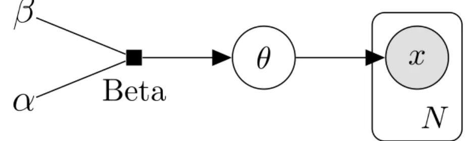
Plate notation helps to indicate sampling in a directed graph (Buntine, 1994). Plates indicate repetition of the nodes inside the plate with the number of repeated nodes shown in the lower corner. For the coin-toss example, if we extend the model to any N coin tosses it would be unwieldy to show that in the style of figure 2.2, but using plate notation we more efficiently show the same information. Plates can be nested.

Beta

α

β

θ

x

N

Figure 2.6: Bayes network with plate notation for determining the bias (θ) of a coin after N flips. The plate is a compact and convenient notation for representing repetition. The repetition is simply a representation of sampling; in this case our model assumes that we draw N samples from θ.

2.8 Some Useful Distributions

The exponential family of distributions is an important and flexible family of distributions that is often used in Bayesian modelling (Bishop, 2006). Notable distributions of the family include the normal, beta, Poisson, Bernoulli, multi-nomial and Dirichlet distributions, amongst others. The exponential family

(48)

provides an expressive set of densities that are broadly applicable and have desirable computational properties.

2.8.1 The Exponential Family

All the distributions in the family have distribution functions in the form over

x and parametrised by η

p(x|η) =h(x)exp

ηTT(x)−a(η) . (2.32) Equation 2.32 is the canonical form for the exponential family. All of the distributions in the exponential family can be written in the canonical form.

η are known as the natural parameters of the distribution; the function a(η) acts to ensure that the distribution is normalised. h(x) is known as the base measure and is a non-negative function that only depends on x.

The exponential family has many desirable properties for Bayesian modelling. All the distributions have a conjugate priors in the exponential family and they have bounded sufficient statistics.

2.8.2 Sufficient Statistics

In the canonical form for the exponential family the sufficient statistic is given by the function T(x). The data contained in the sufficient statistic are all the data required to calculate the statistics (moments) of the distribution, via maximum likelihood or Bayesian methods (Bishop, 2006). An important property of the exponential family is that the dimensions of their sufficient statistics are bounded and do not grow with the amount of data observed. This is important for providing a compact representation for the real-world use of these distributions and ensures that they are computationally feasible for a wide range of models (Hogg & Craig, 1978).

2.8.3 The Normal Distribution

The normal or Gaussian is a well-known member of the exponential family. A continuous distribution for a random variablex, it is parametrised by a mean,

(49)

µ, and a standard deviation, σ (Peebles & Shi, 2001).

N(x;µ, σ2) = p(x|µ, σ2) = √ 1

2πσ2e

(x−µ)2

2σ2 (2.33)

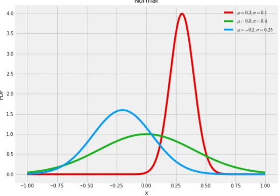
The density has a distinctive bell shape. The mean is a location parameter around which the density is centred and the standard deviation controls the spread of mass around the mean. Some example normals are shown in Figure 2.7, which illustrates how changing the mean and standard deviation changes the location and spread of the PDF.

Figure 2.7: Probability density functions for three normal distributions with differing means and standard deviations. Note how the mean acts to locate the distribution and the standard deviation controls the spread around the mean.

2.8.4 The Binomial Distribution

The binomial distribution is a discrete distribution of the number of successes when carrying out n trials that have a success probability of µ. The binomial

(50)

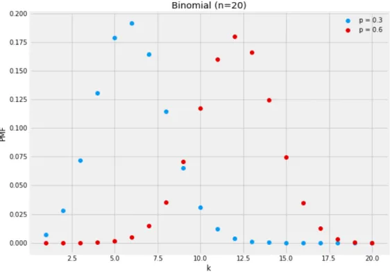
distribution has the following probabilistic mass function: p(k |n, µ) = n k µk(1−µ)n−k (2.34) where: n k = n! k!(n−k)!. (2.35) The binomial can be viewed as giving the probability of observingkheads when flipping a biased coin n times, where the bias µ is the probability of seeing heads. The PMF of various binomials with different success probabilities is shown in Figure 2.8.

Figure 2.8: Probability mass functions for binomials with different success probabilities and twenty trials (n= 20). The binomial is discrete and thus has a PMF.

2.8.5 The Beta Distribution

The beta distribution is a continuous distribution over the range [0,1] and is the conjugate prior to the binomial distribution. It has two parameters,α and

(51)

β, and the PDF is given as:

Beta(x;α, β) = p(x|α, β) = x

α−1₍₁₋_x₎β−1

B(α, β) . (2.36) Where B(α, β) is a normaliser function that ensures that the distribution in-tegrates to 1. The expected value is given by:

E[x] = α

α+β. (2.37)

A sample from a beta distribution is a valid probability, making the beta dis-tribution useful for modelling the likelihood of a binary event, such as success probability or the chance that a coin will come up heads.

2.8.6 The Multinomial Distribution

The multinomial distribution is a discrete distribution over K categories. It is parametrised by a vector p of probabilities where PK

k=1pk = 1 and pk is

the probability of getting category k, and a scalar n which is the number of categories returned from the multinomial. The PMF is:

p(x|n,p) = n! x1!. . . xk! px1 1 . . . p xk k . (2.38)

2.8.7 The Categorical Distribution

The Categorical distribution is simply the multinomial for a single sample. In topic modelling and information retrieval, the Multinomial and Categorical distributions are often used interchangeably (Blei & Lafferty, 2009).

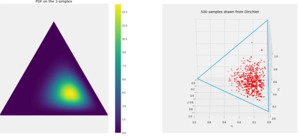
2.8.8 The Dirichlet

The Dirichlet distribution is the multivariate extension to the Beta distribu-tion. The Dirichlet is parametrised by a K-dimensional vector α.

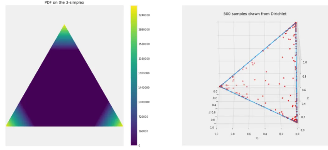
Dir(x;α) = p(x|α) = 1 B(α) K Y k=1 xαk−1 k (2.39)

Where the normaliser is given as:

B(α) = QK k=1Γ(αk) Γ(PK k=1αk) . (2.40)

Recommender systems with Bayesian aspect models and the effect of approximate inference

by

Dylan Verrezen

Thesis presented in partial fulfilment of the requirements

for the degree of Master of Science in Engineering in the

Faculty of Engineering at Stellenbosch University

Abstract

Recommender Systems with Bayesian Aspect Models

and the Effect of Approximate Inference

Uittreksel

Recommender Systems with Bayesian Aspect Models

and the Effect of Approximate Inference

Declaration

Contents

List of Figures

List of Algorithms

Nomenclature

Chapter 1

Introduction

1.1

Motivation

1.2

Background

1.2.1

Ratings Prediction Systems

1.2.2

Matrix Factorisation Models

1.2.3

Topic Models

1.2.4

Ratings Prediction versus Top-N

Recommendation

1.2.5

Bayesian Models and Approximate Inference

1.3

Goals

1.4

Contributions

1.5

Overview

1.5.1

Recommender Systems

1.5.2

Approximate Inference

1.5.3

Key Results and Conclusions

Chapter 2

Bayesian Modelling

2.1

Statistical Modelling

2.1.1

Frequentist and Bayesian Paradigms

2.1.2

Generative Models

2.1.3

Generative Process

2.2

The Rules of Probability

2.2.1

The Sum Rule

2.2.2

The Product Rule

2.3

Bayesian Models

2.3.1

Hierarchical Models

2.3.2

Conditionally Conjugate Models

2.4

Applying Bayes’ Rule

2.4.1

Maximum Likelihood and Maximum a Posteriori

Estimation

2.5

Choice of Priors

2.5.1

Types of Priors

2.5.2

Conjugate Priors

2.5.3

₁

₃