U n i v e r s i t y I n f o r m a t i o n T e c h n o l o g y S e r v i c e s
Regression Models for Ordinal and Nominal Dependent
Variables Using SAS, Stata, LIMDEP, and SPSS
*
Hun Myoung Park, Ph.D.
© 2003-2009
Last modified on September 2009
University Information Technology Services
Center for Statistical and Mathematical Computing
Indiana University
410 North Park Avenue Bloomington, IN 47408
(812) 855-4724 (317) 278-4740
http://www.indiana.edu/~statmath
*
The citation of this document should read: “Park, Hun Myoung. 2009.
Regression Models for Ordinal and
Nominal Dependent Variables Using SAS, Stata, LIMDEP, and SPSS
. Working Paper. The University Information
Technology Services (UITS) Center for Statistical and Mathematical Computing, Indiana University.”
This document summarizes logit and probit regression models for ordinal and nominal
dependent variables and illustrates how to estimate individual models using SAS 9.2, Stata 11,
LIMDEP 9, and SPSS 17.
1.
Introduction
2.
Ordinal Logit and Probit Models
3.
Multinomial Logit Model
4.
Conditional Logit Model
5.
Nested Logit Model
6.
Conclusion
References
1. Introduction
A categorical variable here refers to a variable that is binary, ordinal, or nominal. Event count
data are discrete (categorical) but often treated as continuous variables. When a dependent
variable is categorical, the ordinary least squares (OLS) method can no longer produce the best
linear unbiased estimator (BLUE); that is, OLS is biased and inefficient. Consequently,
researchers have developed various regression models for categorical dependent variables. The
nonlinearity of categorical dependent variable models makes it difficult to fit the models and
interpret their results.
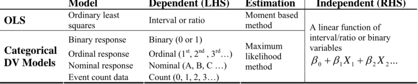
1.1 Regression Models for Categorical Dependent Variables
In categorical dependent variable models, the left-hand side (LHS) variable or dependent
variable is neither interval nor ratio, but rather categorical. The level of measurement and data
generation process (DGP) of a dependent variable determine a proper model for data analysis.
Binary responses (0 or 1) are modeled with binary logit and probit regressions, ordinal
responses (1
st, 2
nd, 3
rd, …) are formulated into (generalized) ordinal logit/probit regressions,
and nominal responses are analyzed by the multinomial logit (probit), conditional logit, or
nested logit model depending on specific circumstances. Independent variables on the
right-hand side (RHS) are interval, ratio, and/or binary (dummy).
Table 1.1 Ordinary Least Squares and Categorical Dependent Variable Models
Model
Dependent (LHS)
Estimation
Independent (RHS)
OLS
Ordinary least
squares
Interval or ratio
Moment based
method
Binary response
Binary (0 or 1)
Ordinal response
Ordinal (1
st, 2
nd, 3
rd…)
Nominal response
Nominal (A, B, C …)
Categorical
DV Models
Event count data
Count (0, 1, 2, 3…)
Maximum
likelihood
method
A linear function of
interval/ratio or binary
variables
...
2 2 1 1 0
X
X
Categorical dependent variable models adopt the maximum likelihood (ML) estimation method,
whereas OLS uses the moment based method. The ML method requires an assumption about
probability distribution functions, such as the logistic function and the complementary log-log
function. Logit models use the standard logistic probability distribution, while probit models
assume the standard normal distribution. This document focuses on logit and probit models
only, excluding regression models for event count data (e.g., negative binomial regression
model and zero-inflated or zero-truncated regression models). Table 1.1 summarizes
categorical dependent variable models in comparison with OLS.
1.2 Logit Models versus Probit Models
How do logit models differ from probit models? The core difference lies in the distribution of
errors (disturbances). In the logit model, errors are assumed to follow the standard logistic
distribution with mean 0 and variance
3
2
,
2)
1
(
)
(
e
e
. The errors of the probit model are
assumed to follow the standard normal distribution,
22
2
1
)
(
e
with variance 1.
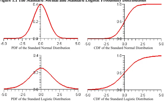
Figure 1.1 The Standard Normal and Standard Logistic Probability Distributions
PDF of the Standard Normal Distribution
CDF of the Standard Normal Distribution
PDF of the Standard Logistic Distribution
CDF of the Standard Logistic Distribution
The probability density function (PDF) of the standard normal probability distribution has a
higher peak and thinner tails than the standard logistic probability distribution (Figure 1.1). The
standard logistic distribution looks as if someone has weighed down the peak of the standard
normal distribution and strained its tails. As a result, the cumulative density function (CDF) of
the standard normal distribution is steeper in the middle than the CDF of the standard logistic
distribution and quickly approaches zero on the left and one on the right.
The two models, of course, produce different parameter estimates. In binary response models,
the estimates of a logit model are roughly
3
times larger than those of the probit model.
These estimators, however, end up with almost the same standardized impacts of independent
variables (Long 1997).
The choice between logit and probit models is more closely related to estimation and
familiarity rather than theoretical and interpretive aspects. In general, logit models reach
convergence fairly well. Although some (multinomial) probit models may take a long time to
reach convergence, a probit model works well for bivariate models. As computing power
improves and new algorithms are developed, importance of this issue is diminishing. For
discussion on choosing logit and probit models, see Cameron and Trivedi (2009: 471-474).
1.3 Estimation in SAS, Stata, LIMDEP, R, and SPSS
SAS provides several procedures for categorical dependent variable models, such as PROC
LOGISTIC, PROBIT, GENMOD, QLIM, MDC, PHREG, and CATMOD. Since these
procedures support various models, a categorical dependent variable model can be estimated by
multiple procedures. For example, you may run a binary logit model using PROC LOGISTIC,
QLIM, GENMOD, and PROBIT. PROC LOGISTIC and PROC PROBIT of SAS/STAT have
been commonly used, but PROC QLIM and PROC MDC of SAS/ETS have advantages over
other procedures. PROC LOGISTIC reports factor changes in the odds and tests key
hypotheses of a model.
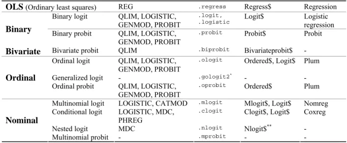
Table 1.2 Procedures and Commands for Categorical Dependent Variable Models
Model
SAS 9.2
Stata 11
LIMDEP 9
SPSS17
OLS (Ordinary least squares)
REG
.regressRegress$ Regression
Binary logit
QLIM, LOGISTIC,
GENMOD, PROBIT
.logit,
.logistic
Logit$ Logistic
regression
Binary
Binary probit
QLIM, LOGISTIC,
GENMOD, PROBIT
.probit
Probit$ Probit
Bivariate
Bivariate probit
QLIM
.biprobitBivariateprobit$ -
Ordinal logit
QLIM, LOGISTIC,
GENMOD, PROBIT
.ologit
Ordered$, Logit$ Plum
Generalized logit
-
.gologit2*- -
Ordinal
Ordinal probit
QLIM, LOGISTIC,
GENMOD, PROBIT
.oprobit
Ordered$ Plum
Multinomial logit
LOGISTIC, CATMOD
.mlogitMlogit$, Logit$
Nomreg
Conditional logit
LOGISTIC, MDC,
PHREG
.clogit
Clogit$, Logit$
Coxreg
Nested logit
MDC
.nlogitNlogit$
**-
Nominal
Multinomial probit -
.mprobit- -
* A user-written command written by Williams (2005)
** The
Nlogit$
command is supported by NLOGIT, a stand-alone package, which is sold separately.
The QLIM (Qualitative and LImited dependent variable Model) procedure analyzes various
categorical and limited dependent variable regression models such as censored, truncated, and
sample-selection models. PROC QLIM also handles Box-Cox regression and the bivariate
probit model. The MDC (Multinomial Discrete Choice) procedure can estimate conditional
logit and nested logit models.
Another advantage of using SAS is the Output Delivery System (ODS), which makes it easy to
manage SAS output. ODS enables users to redirect the output to HTML (Hypertext Markup
Language) and RTF (Rich Text Format) formats. Once SAS output is generated in a HTML
document, users can easily handle tables and graphics especially when copying and pasting
them into a wordprocessor document.
Unlike SAS, Stata has individualized commands for corresponding categorical dependent
variable models. For example, the
.logit
and
.probit
commands respectively fit the binary
logit and probit models, while
.mlogit
and
.nlogit
estimate the mulitinomial logit and
nested logit models. Stata enables users to perform post-hoc analyses such as marginal effects
and discrete changes in an easy manner.
The LIMDEP
Logit$
and
Probit$
commands support a variety of categorical dependent
variable models that are addressed in Greene’s
Econometric Analysis
(2003). The output format
of LIMDEP 9 is slightly different from that of previous version, but key statistics remain
unchanged. The nested logit model and multinomial probit model in LIMDEP are estimated by
NLOGIT, a separate package. In R,
glm()
fits binary logit and probit models in the object-
oriented programming concept. SPSS also supports some categorical dependent variable
models and its output is often messy and hard to read. Stata and R are case-sensitive, but SAS,
LIMDEP, and SPSS are not. Table 1.2 summarizes the procedures and commands used for
categorical dependent variable models.
1. 4 Long and Freese’s SPost
Stata users may benefit from user-written commands such as J. Scott Long and Jeremy Freese’s
SPost. This collection of user-written commands conducts many follow-up analyses of various
categorical dependent variable models including event count data models (See section 2.2).
In order to install SPost, execute the following commands consecutively. Visit J. Scott Long’s
Web site at http://www.indiana.edu/~jslsoc/ to get further information.
. net from http://www.indiana.edu/~jslsoc/stata/ . net install spost9_ado, replace
. net get spost9_do, replace
If a Stata command, function, or user-written command does not work in version 11, run
the
.version
command to switch the interpreter to old one and execute that command again.
For example,
normal()
was
norm()
in old versions. Also you may update Stata or reinstall
user-written models to get their latest version installed.
. version 9
You may use Vincent Kang Fu’s
gologit
(1998) and Richard Williams’
gologit2
(2005) for
the generalized ordinal logit model.
.mfx2
is a related command written by Williams to
compute marginal effects (discrete changes) in (generalized) ordinal logit and multinomial logit
models. Visit http://www.nd.edu/~rwilliam/gologit2/tsfaq.html for more information.
. net install gologit, from(http://www.stata.com/users/jhardin) replace . ssc install gologit2, replace
2. Ordinal Logit and Probit Regression Models
Suppose we have an ordinal dependent variable such as religious intensity (0=no religion,
1=somewhat strong, 2=not very strong, and 3=strong). Ordinal logit and probit models have the
parallel regression assumption or proportional odds assumption, which in practice is often
violated.
2.1 Ordinal Logit Model in Stata (.ologit)
Stata has
.ologit
and
.oprobit
commands to estimate ordinal logit and probit regression
models, respectively. Their output looks like the result of
.logit
except for cut points and the
intercept. Stata estimates
m,
/cut1
,
/cut2
, and
/cut3
, assuming
0
0
(Long and Freese
2003: 148-149). Accordingly, the output below does not report the intercept. By contrast,
PROC QLIM, PROC PROBIT, and LIMDEP have different parameterization and assume
0
1
; therefore, (
0-/cut1)
is reported as their intercept.
. use http://www.indiana.edu/~statmath/stat/all/cdvm/gss_cdvm.dta, clear . ologit belief educate income age male www
Iteration 0: log likelihood = -1499.6929 Iteration 1: log likelihood = -1480.3168 Iteration 2: log likelihood = -1480.2738 Iteration 3: log likelihood = -1480.2738
Ordered logistic regression Number of obs = 1174 LR chi2(5) = 38.84 Prob > chi2 = 0.0000 Log likelihood = -1480.2738 Pseudo R2 = 0.0129
--- belief | Coef. Std. Err. z P>|z| [95% Conf. Interval] ---+--- educate | -.0020145 .0220039 -0.09 0.927 -.0451414 .0411124 income | -.0059213 .0089976 -0.66 0.510 -.0235563 .0117137 age | .0186456 .0042123 4.43 0.000 .0103897 .0269015 male | -.4661952 .1085422 -4.30 0.000 -.6789339 -.2534564 www | .1264832 .1357087 0.93 0.351 -.1395009 .3924673 ---+--- /cut1 | -1.183894 .3674989 -1.904178 -.463609 /cut2 | -.4989643 .3648623 -1.214081 .2161526 /cut3 | 1.186547 .366256 .4686988 1.904396 ---
The model fairly fits the date although only age and gender are statistically significant.
SPost
.fitstat
returns a list of goodness-of-fit measures.
D(1166)
indicates that this model
estimates eight parameters (five regressors and three cut points): 1,166=1,174-8.
. fitstat
Measures of Fit for ologit of belief
Log-Lik Intercept Only: -1499.693 Log-Lik Full Model: -1480.274 D(1166): 2960.548 LR(5): 38.838 Prob > LR: 0.000 McFadden's R2: 0.013 McFadden's Adj R2: 0.008 ML (Cox-Snell) R2: 0.033 Cragg-Uhler(Nagelkerke) R2: 0.035 McKelvey & Zavoina's R2: 0.033
Count R2: 0.407 Adj Count R2: 0.031 AIC: 2.535 AIC*n: 2976.548 BIC: -5280.941 BIC': -3.497 BIC used by Stata: 3017.093 AIC used by Stata: 2976.548
Ordinal logit and probit models are not as easy to interpret the output as binary response
models. Factor changes in the odds are better for interpretation than marginal effects and
discrete changes in the ordinal logit model.
The factor change in the odds of a lower versus a
higher outcome
is exp(b) in binary response models (0 versus 1), but exp(-b) in the ordinal logit
model. For the sake of convenience in interpretation, however,
the factor change in the odds of
a higher outcome compared to a lower outcome
, exp(b), can be considered an alternative (Long
and Freese 2003: 165-168). Also see Long (1997: 138-140). Although numerically different,
both factor changes are equivalent.
The following
.listcoef
produces factor changes in the odds of a higher compared to a lower
outcome. For instance, the factor change in the odds of age is 1.0188=exp(b)=exp(.0187)=
=1/exp(-.0187)=1/.9815, holding all other covariates constant. For a unit increase in age,
the
odds of having stronger religious belief
change (increase in this case) by the factor of 1.0188,
holding all other variables constant. For a standard deviation increase in age, the odds of having
stronger religious belief compared to weaker belief increase by the factor of 1.2840=
exp(.01865*13.4071)=1/exp(-.01865*13.4071)=1/.7788. The odds of having stronger religious
belief are .6274=exp(-.4662)=1/exp(.4662)=1/1.5939 times smaller for men than for women.
. listcoef, help
ologit (N=1174): Factor Change in Odds Odds of: >m vs <=m
--- belief | b z P>|z| e^b e^bStdX SDofX ---+--- educate | -0.00201 -0.092 0.927 0.9980 0.9948 2.5697 income | -0.00592 -0.658 0.510 0.9941 0.9640 6.1943 age | 0.01865 4.427 0.000 1.0188 1.2840 13.4071 male | -0.46620 -4.295 0.000 0.6274 0.7929 0.4978 www | 0.12648 0.932 0.351 1.1348 1.0533 0.4108 --- b = raw coefficient
z = z-score for test of b=0 P>|z| = p-value for z-test
e^b = exp(b) = factor change in odds for unit increase in X e^bStdX = exp(b*SD of X) = change in odds for SD increase in X SDofX = standard deviation of X
The
reverse
option in
.listcoef
computes factor changes in the odds of a lower outcome
compared to a higher outcome. The factor changes in the odds of having weaker religious belief
with respect to age is .9815=exp(-b)=exp(-.0187)=1/1.0188. For a unit increase in age, the
odds
of having weaker belief
decrease by a factor of .9815. The odds of having weaker religious
belief are 1.5939 = exp(-(-.4662)) = 1/.6274 times larger for men than for women, holding all
other variables constant.
. listcoef, reverse
ologit (N=1174): Factor Change in Odds Odds of: <=m vs >m
--- belief | b z P>|z| e^b e^bStdX SDofX ---+--- educate | -0.00201 -0.092 0.927 1.0020 1.0052 2.5697 income | -0.00592 -0.658 0.510 1.0059 1.0374 6.1943 age | 0.01865 4.427 0.000 0.9815 0.7788 13.4071 male | -0.46620 -4.295 0.000 1.5939 1.2612 0.4978 www | 0.12648 0.932 0.351 0.8812 0.9494 0.4108 ---
Alternatively, you may also compute the percentage changes in the odds using the
percent
option. The odds of having stronger religious belief are 37.3 percent smaller for men than for
woman, holding all other variables constant.
. listcoef, percent help
ologit (N=1174): Percentage Change in Odds Odds of: >m vs <=m --- belief | b z P>|z| % %StdX SDofX ---+--- educate | -0.00201 -0.092 0.927 -0.2 -0.5 2.5697 income | -0.00592 -0.658 0.510 -0.6 -3.6 6.1943 age | 0.01865 4.427 0.000 1.9 28.4 13.4071 male | -0.46620 -4.295 0.000 -37.3 -20.7 0.4978 www | 0.12648 0.932 0.351 13.5 5.3 0.4108 --- b = raw coefficient
z = z-score for test of b=0 P>|z| = p-value for z-test
% = percent change in odds for unit increase in X %StdX = percent change in odds for SD increase in X SDofX = standard deviation of X
Marginal effects (discrete changes) are used to interpret the output substantively. Use
either
.mfx
or
.prchange
with, if you want, particular reference points other than the default
means of covariates specified.
.mfx
reports standard errors of marginal effects and discrete
changes, but
.prchange
does not.
.prchange
reports the predicted probability of having no religion (
belief=0
) and list marginal
effects (discrete changes for binary variables). For female WWW users at the average age of 41
who graduated a college (16 years of education) and have the average family income of 25
thousand dollars (see reference points under the last column
x
below), the predicted probability
of having no religion is 12.98 percent.
. mfx, at(mean educate=16 male=0 www=1)
Marginal effects after ologit y = Pr(belief==0) (predict) = .12983744
--- variable | dy/dx Std. Err. z P>|z| [ 95% C.I. ] X ---+--- educate | .0002276 .00249 0.09 0.927 -.004655 .005111 16 income | .000669 .00102 0.66 0.510 -.001322 .002659 24.6486 age | -.0021066 .00049 -4.27 0.000 -.003075 -.001139 41.3075 male*| .0622968 .01503 4.15 0.000 .032845 .091748 0 www*| -.014971 .0166 -0.90 0.367 -.047509 .017567 1 --- (*) dy/dx is for discrete change of dummy variable from 0 to 1
Marginal effects and discrete changes are more intuitive than factor changes in the odds. For 10
unit increase in age from its mean 41, the probability of having no religion is expected to
decrease by 2.1 percent (.21*10), holding all other variables constant at the reference points.
Men are 6.23 percent more likely than women to have no religion at the same reference points.
.prchange
reports predicted probabilities of four religious intensity and produces marginal
effects (
-+1/2
or
MargEfct
) and discrete changes (
0->1
) of covariates in probabilities of all
four outcomes. This command computes marginal effects for a standard deviation change (
-+sd/2
) as well.
. prchange age male, x(educate=16 male=0 www=1) rest(mean)
ologit: Changes in Probabilities for belief age
Avg|Chg| No_relig Somewhat Not_very Strong Min->Max .1509029 -.12637663 -.07334894 -.10208026 .30180579 -+1/2 .00220756 -.00210658 -.00117922 -.00112933 .00441512 -+sd/2 .02956489 -.02826677 -.01577979 -.01508322 .05912977 MargEfct .00220758 -.00210658 -.00117923 -.00112935 .00441516 male
Avg|Chg| No_relig Somewhat Not_very Strong 0->1 .05150692 .06229679 .02986491 .01085213 -.10301384 No_relig Somewhat Not_very Strong
Pr(y|x) .12983744 .09854499 .3865383 .38507926 educate income age male www x= 16 24.6486 41.3075 0 1 sd_x= 2.56971 6.19427 13.4071 .497765 .410755
Find the same marginal effect of age -.0021 at the
MargEfct
or
-+1/2
row under the label
No_relig
. Interestingly, only marginal effects on having strong intensity are positive. For a
standard deviation increases in age (13.4071) from the mean 41, the probability of having
strong religious belief is expected to increase by 5.91 percent, holding all other variables
constant at their reference points. By contrast, signs of discrete changes of gender are opposite.
The probability that men WWW users have strong belief is 10.30 percent lower than that of
women counterparts, holding all other variables at their reference points.
Williams’
.mfx2
is very useful especially for ordinal and multinomial response models. This
command produces marginal effects (discrete changes) and their standard errors for all
outcomes, whereas
.mfx
reports marginal effects for the first outcome (0 in this case) only. But
they share the same output format. Therefore,
.prchange
in fact summarizes the output
of
.mfx2
. Compare the following output with what
.prchange
produced above.
. mfx2, at(mean educate=16 male=0 www=1)
Frequencies for belief... Religious |
Intensity | Freq. Percent Cum. ---+--- No religion | 192 16.35 16.35 Somewhat strong | 134 11.41 27.77 Not very strong | 456 38.84 66.61 Strong | 392 33.39 100.00 ---+---
Total | 1,174 100.00
Computing marginal effects after ologit for belief == 0... Marginal effects after ologit
y = Pr(belief==0) (predict, o(0)) = .12983744
--- variable | dy/dx Std. Err. z P>|z| [ 95% C.I. ] X ---+--- educate | .0002276 .00249 0.09 0.927 -.004655 .005111 16 income | .000669 .00102 0.66 0.510 -.001322 .002659 24.6486 age | -.0021066 .00049 -4.27 0.000 -.003075 -.001139 41.3075 male*| .0622968 .01503 4.15 0.000 .032845 .091748 0 www*| -.014971 .0166 -0.90 0.367 -.047509 .017567 1 --- (*) dy/dx is for discrete change of dummy variable from 0 to 1
Computing marginal effects after ologit for belief == 1... Marginal effects after ologit
y = Pr(belief==1) (predict, o(1)) = .09854499
--- variable | dy/dx Std. Err. z P>|z| [ 95% C.I. ] X ---+--- educate | .0001274 .00139 0.09 0.927 -.002602 .002857 16 income | .0003745 .00057 0.66 0.511 -.000742 .001491 24.6486 age | -.0011792 .00028 -4.17 0.000 -.001733 -.000625 41.3075 male*| .0298649 .0073 4.09 0.000 .015564 .044166 0 www*| -.0080795 .00874 -0.92 0.355 -.025211 .009052 1 --- (*) dy/dx is for discrete change of dummy variable from 0 to 1
Computing marginal effects after ologit for belief == 2... Marginal effects after ologit
y = Pr(belief==2) (predict, o(2)) = .3865383
--- variable | dy/dx Std. Err. z P>|z| [ 95% C.I. ] X ---+--- educate | .000122 .00132 0.09 0.927 -.002472 .002716 16 income | .0003586 .00055 0.65 0.517 -.000727 .001444 24.6486 age | -.0011294 .00036 -3.15 0.002 -.001833 -.000426 41.3075 male*| .0108521 .0057 1.90 0.057 -.000329 .022033 0 www*| -.006432 .00619 -1.04 0.299 -.018568 .005704 1 --- (*) dy/dx is for discrete change of dummy variable from 0 to 1
Computing marginal effects after ologit for belief == 3...
Marginal effects after ologit
y = Pr(belief==3) (predict, o(3)) = .38507927
--- variable | dy/dx Std. Err. z P>|z| [ 95% C.I. ] X ---+--- educate | -.000477 .00521 -0.09 0.927 -.010682 .009728 16 income | -.0014021 .00213 -0.66 0.511 -.00558 .002776 24.6486 age | .0044152 .001 4.41 0.000 .002455 .006375 41.3075 male*| -.1030138 .02374 -4.34 0.000 -.149547 -.056481 0 www*| .0294825 .03126 0.94 0.346 -.031777 .090743 1 --- (*) dy/dx is for discrete change of dummy variable from 0 to 1
Now, move on to the interpretation using predicted probabilities. Like
.prchange
and
.mfx2
,
probability of no religion is 12.98, 9.85 for somewhat strong, 38.65 for not very strong, and
38.51 for strong religious belief.
. prvalue, x(educate=16 male=0 www=1) rest(mean)
ologit: Predictions for belief Confidence intervals by delta method
95% Conf. Interval Pr(y=No_relig|x): 0.1298 [ 0.1063, 0.1533] Pr(y=Somewhat|x): 0.0985 [ 0.0805, 0.1166] Pr(y=Not_very|x): 0.3865 [ 0.3577, 0.4154] Pr(y=Strong|x): 0.3851 [ 0.3437, 0.4265] educate income age male www x= 16 24.648637 41.307496 0 1
The
.prtab
command constructs the tables of predicted probabilities for combinations of
different values of independent variables. The following tables suggest that gender appears to
make difference in religious intensity.
. prtab male www, x(educate=16 male=0 www=1) rest(mean)
ologit: Predicted probabilities for belief
Predicted probability of outcome 0 (No_religion) ---
| WWW Use Gender | Non-users Users ---+--- Female | 0.1448 0.1298 Male | 0.2125 0.1921 ---
Predicted probability of outcome 1 (Somewhat_strong) ---
| WWW Use Gender | Non-users Users ---+--- Female | 0.1066 0.0985 Male | 0.1362 0.1284 ---
Predicted probability of outcome 2 (Not_very_strong) ---
| WWW Use Gender | Non-users Users ---+--- Female | 0.3930 0.3865 Male | 0.3941 0.3974 ---
Predicted probability of outcome 3 (Strong) ---
| WWW Use Gender | Non-users Users ---+--- Female | 0.3556 0.3851 Male | 0.2572 0.2821 ---
x= 16 24.648637 41.307496 0 1
SPost
.prgen
is very useful when visualizing predicted probabilities. The following commands
produce a series of predicted probabilities as age changes from 18 to 92.
ncases(20)
computes
predicted probabilities at the 20 different points of age, holding other independent variables at
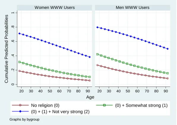
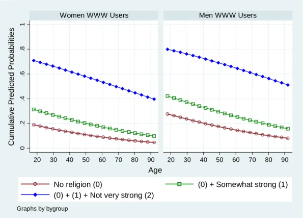
the reference points. See the attached Stata script for data manipulation for Figure 2.1. As we
found in the above tables, women are more likely to have strong belief and less likely to have
no religions than men.
. prgen age, from(18) to(92) ncases(20) x(educate=16 male=1 www=1) rest(mean) gen(Logit_age1)
ologit: Predicted values as age varies from 18 to 92. educate income age male www x= 16 24.648637 41.307496 1 1
. prgen age, from(18) to(92) ncases(20) x(educate=16 male=0 www=1) rest(mean) gen(Logit_age0)
ologit: Predicted values as age varies from 18 to 92. educate income age male www x= 16 24.648637 41.307496 0 1
Figure 2.1 Predicted Probabilities of Religious Intensity (Ordinal Logit Model)
0 .2 .4 .6 .8 1 20 30 40 50 60 70 80 90 20 30 40 50 60 70 80 90
Women WWW Users
Men WWW Users
No religion (0)
(0) + Somewhat strong (1)
(0) + (1) + Not very strong (2)
C
u
m
u
la
ti
v
e
P
red
ic
te
d
P
rob
ab
ilit
ie
s
Age
Graphs by bygroup2.2 Ordinal Probit Model in Stata (.oprobit)
Let us fit the ordinal probit model using the same specification. Logit and probit models
produce similar parameter estimates and goodness-of-fit measures. For example, their
likelihood ratios are 38.84 versus 40.13 and pseudo R
2are .0129 versus .0134, respectively.
. oprobit belief educate income age male www
Iteration 0: log likelihood = -1499.6929 Iteration 1: log likelihood = -1479.63 Iteration 2: log likelihood = -1479.6279 Iteration 3: log likelihood = -1479.6279
Ordered probit regression Number of obs = 1174 LR chi2(5) = 40.13 Prob > chi2 = 0.0000 Log likelihood = -1479.6279 Pseudo R2 = 0.0134 --- belief | Coef. Std. Err. z P>|z| [95% Conf. Interval] ---+--- educate | -.0015194 .0130701 -0.12 0.907 -.0271362 .0240974 income | -.0027382 .0053709 -0.51 0.610 -.0132649 .0077886 age | .0109693 .0024755 4.43 0.000 .0061175 .0158211 male | -.290305 .0646295 -4.49 0.000 -.4169764 -.1636335 www | .0642404 .0809186 0.79 0.427 -.0943572 .2228379 ---+--- /cut1 | -.7138045 .2182722 -1.14161 -.2859989 /cut2 | -.3178217 .2172398 -.7436038 .1079604 /cut3 | .7199238 .217734 .293173 1.146675 --- . fitstat
Measures of Fit for oprobit of belief
Log-Lik Intercept Only: -1499.693 Log-Lik Full Model: -1479.628 D(1166): 2959.256 LR(5): 40.130 Prob > LR: 0.000 McFadden's R2: 0.013 McFadden's Adj R2: 0.008 ML (Cox-Snell) R2: 0.034 Cragg-Uhler(Nagelkerke) R2: 0.036 McKelvey & Zavoina's R2: 0.040
Variance of y*: 1.041 Variance of error: 1.000 Count R2: 0.414 Adj Count R2: 0.042 AIC: 2.534 AIC*n: 2975.256 BIC: -5282.233 BIC': -4.789 BIC used by Stata: 3015.801 AIC used by Stata: 2975.256
In a probit model,
.listcoef
produces standardized coefficients instead of factor changes (or
percent changes) of the odds.
. listcoef, help
oprobit (N=1174): Unstandardized and Standardized Estimates Observed SD: 1.044809
Latent SD: 1.020498
--- belief | b z P>|z| bStdX bStdY bStdXY SDofX ---+--- educate | -0.00152 -0.116 0.907 -0.0039 -0.0015 -0.0038 2.5697 income | -0.00274 -0.510 0.610 -0.0170 -0.0027 -0.0166 6.1943 age | 0.01097 4.431 0.000 0.1471 0.0107 0.1441 13.4071 male | -0.29030 -4.492 0.000 -0.1445 -0.2845 -0.1416 0.4978 www | 0.06424 0.794 0.427 0.0264 0.0630 0.0259 0.4108 --- b = raw coefficient
z = z-score for test of b=0 P>|z| = p-value for z-test
bStdX = x-standardized coefficient bStdY = y-standardized coefficient bStdXY = fully standardized coefficient SDofX = standard deviation of X
Let us compute predicted probabilities and marginal effects (discrete changes) at the same
reference points. The following
.mfx
command reports that 12.73 percent of female WWW
users have no religion (12.98 percent in the logit model above).
. mfx, at(mean educate=16 male=0 www=1)
Marginal effects after oprobit y = Pr(belief==0) (predict) = .12727708
--- variable | dy/dx Std. Err. z P>|z| [ 95% C.I. ] X ---+--- educate | .0003167 .00273 0.12 0.908 -.005037 .00567 16 income | .0005708 .00112 0.51 0.610 -.001622 .002764 24.6486 age | -.0022867 .00053 -4.28 0.000 -.003335 -.001238 41.3075 male*| .070649 .01616 4.37 0.000 .038981 .102317 0 www*| -.0138841 .01793 -0.77 0.439 -.04903 .021262 1 --- (*) dy/dx is for discrete change of dummy variable from 0 to 1
.prvalue
reports other predicted probabilities as well: 10.14 percent for somewhat strong,
38.71 for not very strong, and 38.42 for the strong religious belief (9.85, 38.65, and 38.51 in the
logit model above).
. prvalue, x(educate=16 male=0 www=1) rest(mean)
oprobit: Predictions for belief Confidence intervals by delta method
95% Conf. Interval Pr(y=No_relig|x): 0.1273 [ 0.1028, 0.1518] Pr(y=Somewhat|x): 0.1014 [ 0.0823, 0.1204] Pr(y=Not_very|x): 0.3871 [ 0.3561, 0.4182] Pr(y=Strong|x): 0.3842 [ 0.3438, 0.4247] educate income age male www x= 16 24.648637 41.307496 0 1
The following output of
.prchange
reports that marginal effect and discrete change on having
strong belief are .42 percent for age and -10.49 percent for gender, which are respectively very
similar to .44 and -10.30 percent in the logit model above.
. prchange age male, x(educate=16 male=0 www=1) rest(mean)
oprobit: Changes in Probabilities for belief
age
Avg|Chg| No_relig Somewhat Not_very Strong Min->Max .14324967 -.13683906 -.06736732 -.08229297 .28649932 -+1/2 .00209527 -.00228667 -.00103298 -.00087088 .00419053 -+sd/2 .02806862 -.03066584 -.0138232 -.01164818 .05613723 MargEfct .00209528 -.00228667 -.00103299 -.00087091 .00419057 male
Avg|Chg| No_relig Somewhat Not_very Strong 0->1 .05242721 .07064901 .02597284 .00823256 -.1048544 No_relig Somewhat Not_very Strong
Pr(y|x) .12727708 .10135041 .38713527 .38423723 educate income age male www x= 16 24.6486 41.3075 0 1
sd_x= 2.56971 6.19427 13.4071 .497765 .410755
Williams’
.mfx2
produces predicted probabilities, marginal effects (discrete changes), and
standard errors for all four categories in a single command. Compare the output of
.prchange
and
.mfx2
.
. mfx2, at(mean educate=16 male=0 www=1)
Frequencies for belief... Religious |
Intensity | Freq. Percent Cum. ---+--- No religion | 192 16.35 16.35 Somewhat strong | 134 11.41 27.77 Not very strong | 456 38.84 66.61 Strong | 392 33.39 100.00 ---+--- Total | 1,174 100.00
Computing marginal effects after oprobit for belief == 0... Marginal effects after oprobit
y = Pr(belief==0) (predict, o(0)) = .12727708
--- variable | dy/dx Std. Err. z P>|z| [ 95% C.I. ] X ---+--- educate | .0003167 .00273 0.12 0.908 -.005037 .00567 16 income | .0005708 .00112 0.51 0.610 -.001622 .002764 24.6486 age | -.0022867 .00053 -4.28 0.000 -.003335 -.001238 41.3075 male*| .070649 .01616 4.37 0.000 .038981 .102317 0 www*| -.0138841 .01793 -0.77 0.439 -.04903 .021262 1 --- (*) dy/dx is for discrete change of dummy variable from 0 to 1
Computing marginal effects after oprobit for belief == 1... Marginal effects after oprobit
y = Pr(belief==1) (predict, o(1)) = .10135041
--- variable | dy/dx Std. Err. z P>|z| [ 95% C.I. ] X ---+--- educate | .0001431 .00123 0.12 0.907 -.002269 .002555 16 income | .0002579 .00051 0.51 0.611 -.000734 .00125 24.6486 age | -.001033 .00025 -4.16 0.000 -.00152 -.000546 41.3075 male*| .0259728 .00613 4.24 0.000 .013958 .037987 0 www*| -.0060148 .00755 -0.80 0.426 -.020822 .008792 1 --- (*) dy/dx is for discrete change of dummy variable from 0 to 1
Computing marginal effects after oprobit for belief == 2... Marginal effects after oprobit
y = Pr(belief==2) (predict, o(2)) = .38713527
--- variable | dy/dx Std. Err. z P>|z| [ 95% C.I. ] X ---+--- educate | .0001206 .00103 0.12 0.907 -.001895 .002136 16 income | .0002174 .00043 0.50 0.614 -.000627 .001062 24.6486 age | -.0008709 .00028 -3.15 0.002 -.001412 -.000329 41.3075 male*| .0082326 .00456 1.81 0.071 -.000701 .017166 0 www*| -.0043953 .00504 -0.87 0.383 -.01428 .005489 1 --- (*) dy/dx is for discrete change of dummy variable from 0 to 1
Computing marginal effects after oprobit for belief == 3... Marginal effects after oprobit
y = Pr(belief==3) (predict, o(3)) = .38423723
--- variable | dy/dx Std. Err. z P>|z| [ 95% C.I. ] X ---+--- educate | -.0005804 .00499 -0.12 0.907 -.01036 .0092 16 income | -.001046 .00205 -0.51 0.610 -.005069 .002977 24.6486 age | .0041906 .00095 4.43 0.000 .002335 .006046 41.3075 male*| -.1048544 .02315 -4.53 0.000 -.150222 -.059487 0 www*| .0242943 .03037 0.80 0.424 -.035234 .083822 1 --- (*) dy/dx is for discrete change of dummy variable from 0 to 1
You may present predicted probabilities computed at different values of key variables. The
following predicted probabilities suggest that women are less likely to have no religion (12.73
versus 19.79 percent for WWW users) and more likely to have strong belief (38.42 versus
27.94 percent for WWW users) than men, and that there is no substantial difference in religious
intensity between WWW users and non-users. Find the same predicted probabilities (12.73,
10.14, 38.71, and 38.42) in the following four tables generated by
.prtab
.
. prtab male www, x(educate=16 male=0 www=1) rest(mean)
oprobit: Predicted probabilities for belief Predicted probability of outcome 0 (No_religion)
--- | WWW Use Gender | Non-users Users ---+--- Female | 0.1412 0.1273 Male | 0.2163 0.1979 ---
Predicted probability of outcome 1 (Somewhat_strong) ---
| WWW Use Gender | Non-users Users ---+--- Female | 0.1074 0.1014 Male | 0.1324 0.1273 ---
Predicted probability of outcome 2 (Not_very_strong) ---
| WWW Use Gender | Non-users Users ---+--- Female | 0.3915 0.3871 Male | 0.3931 0.3954 ---
Predicted probability of outcome 3 (Strong) ---
| WWW Use Gender | Non-users Users ---+--- Female | 0.3599 0.3842 Male | 0.2582 0.2794 ---
educate income age male www x= 16 24.648637 41.307496 0 1
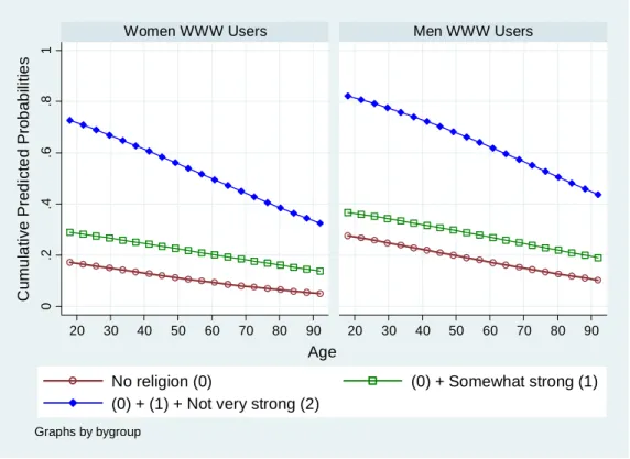
Visualizing cumulative predicted probabilities is another effective way to present the result
(Figure 2.2). Three curves segment each plane into four parts from no religion (bottom),
somewhat strong, not very strong, to strong belief (top). Strong belief holds a larger portion in
the women’s plane than in the men’s. Men are more likely to have no religion than women
when controlling age and other covariates. As people get older, they are more likely to have
strong belief and less likely to have no religion. Age does not appear to affect somewhat strong
and not very strong categories significantly. Figure 2.1 and 2.2 are almost identical.
The following
.prgen
produces a series of predicted probabilities as age changes from 18 to 92.
ncases(20)
computes predicted probabilities at the 20 different points of age, holding other
independent variables at the reference points.
. prgen age, from(18) to(92) ncases(20) x(educate=16 male=1 www=1) rest(mean) gen(Page1)
oprobit: Predicted values as age varies from 18 to 92.
educate income age male www x= 16 24.648637 41.307496 1 1
. prgen age, from(18) to(92) ncases(20) x(educate=16 male=0 www=1) rest(mean) gen(Page0)
oprobit: Predicted values as age varies from 18 to 92. educate income age male www x= 16 24.648637 41.307496 0 1
Figure 2.2 Predicted Probabilities of Religious Intensity (Ordinal Probit Model)
0 .2 .4 .6 .8 1 20 30 40 50 60 70 80 90 20 30 40 50 60 70 80 90
Women WWW Users
Men WWW Users
No religion (0)
(0) + Somewhat strong (1)
(0) + (1) + Not very strong (2)
C
u
m
u
la
ti
v
e
P
red
ic
te
d P
rob
a
b
ilit
ie
s
Age
Graphs by bygroup2.3 Parallel Regression Assumption and Generalized Ordinal Logit Models
The
.brant
command of SPost conducts the Brant test after the
.ologit
command. This
command tests the parallel regression assumption (or proportional odds assumption) of the
ordinal logit regression model. The test suggests that age and gender may have different slopes
across categories. The large chi-squared of 21.94 rejects the null hypothesis of the parallel
regression assumption at the .05 level.
. quietly ologit belief educate income age male www . brant, detail
Estimated coefficients from j-1 binary regressions y>0 y>1 y>2 educate -.01683738 -.01987509 .01376747 income .00437285 -.00678136 -.00665741 age .01549009 .01092697 .02364093 male -.6489834 -.34446179 -.51696936 www -.03895167 .2059211 .10840812 _cons 1.4968083 .96044435 -1.5775835 Brant Test of Parallel Regression Assumption Variable | chi2 p>chi2 df ---+--- All | 21.94 0.015 10 ---+--- educate | 1.46 0.482 2 income | 1.67 0.434 2 age | 6.59 0.037 2 male | 7.99 0.018 2 www | 2.66 0.264 2 ---
A significant test statistic provides evidence that the parallel regression assumption has been violated.
The parallel regression assumption is often violated. If this is the case, you may use the
multinomial logit model or estimate the generalized ordinal logit model using either
the
.gologit
command written by Fu (1998) or the
.gologit2
command by Williams (2005).
Notice that Fu’s command does not impose the restriction of
(
j
x
j)
(
j1
x
j1)
(Long’s class note 2003). Let us begin with Fu’s
.gologit
.
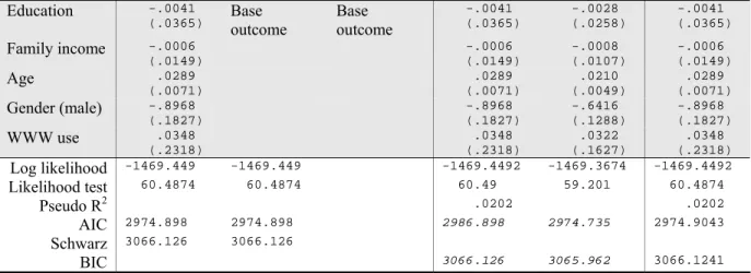
. gologit belief educate income age male www
Iteration 0: Log Likelihood = -1499.6929 Iteration 1: Log Likelihood = -1476.9406 Iteration 2: Log Likelihood = -1469.3715 Iteration 3: Log Likelihood = -1469.3215 Iteration 4: Log Likelihood = -1469.3214 Iteration 5: Log Likelihood = -1469.3214
Generalized Ordered Logit Estimates Number of obs = 1174 Model chi2(15) = 60.74 Prob > chi2 = 0.0000 Log Likelihood = -1469.3214457 Pseudo R2 = 0.0203 --- belief | Coef. Std. Err. z P>|z| [95% Conf. Interval] ---+---
mleq1 | educate | -.0215025 .0313129 -0.69 0.492 -.0828747 .0398696 income | -.0011176 .0123599 -0.09 0.928 -.0253425 .0231073 age | .0165176 .0062489 2.64 0.008 .00427 .0287652 male | -.6447443 .1602963 -4.02 0.000 -.9589192 -.3305693 www | -.0326311 .2046955 -0.16 0.873 -.433827 .3685648 _cons | 1.651383 .5292113 3.12 0.002 .6141477 2.688618 ---+--- mleq2 | educate | -.0226758 .0270061 -0.84 0.401 -.0756068 .0302553 income | -.006108 .0109703 -0.56 0.578 -.0276093 .0153933 age | .0108099 .005133 2.11 0.035 .0007494 .0208705 male | -.3500519 .131329 -2.67 0.008 -.607452 -.0926518 www | .2117636 .1658317 1.28 0.202 -.1132606 .5367877 _cons | .9875713 .4478875 2.20 0.027 .1097279 1.865415 ---+--- mleq3 | educate | .0160895 .0256324 0.63 0.530 -.0341492 .0663282 income | -.0072066 .0106401 -0.68 0.498 -.0280609 .0136477 age | .0238357 .0048312 4.93 0.000 .0143667 .0333046 male | -.5126078 .1285168 -3.99 0.000 -.7644962 -.2607194 www | .1149432 .1613481 0.71 0.476 -.2012932 .4311796 _cons | -1.612449 .4276243 -3.77 0.000 -2.450577 -.7743211 ---
Williams’
.gologit2
fits another version of the generalized ordinal logit regression model.
autofit
tests if the proportional odds assumption is satisfied. This test reports that education,
family income, and WWW use have parallel lines (slopes) but age and gender may not. The
Wald test does not reject the null hypothesis of the parallel regression assumption at the .05
level. This result conflicts with the Brant test that rejects the null hypothesis.
. gologit2 belief educate income age male www, autofit
--- Testing parallel lines assumption using the .05 level of significance...
Step 1: Constraints for parallel lines imposed for income (P Value = 0.7820) Step 2: Constraints for parallel lines imposed for educate (P Value = 0.3893) Step 3: Constraints for parallel lines imposed for www (P Value = 0.2635) Step 4: Constraints for parallel lines are not imposed for
age (P Value = 0.01066) male (P Value = 0.01923)
Wald test of parallel lines assumption for the final model: ( 1) [No_religion]income - [Somewhat_strong]income = 0 ( 2) [No_religion]educate - [Somewhat_strong]educate = 0 ( 3) [No_religion]www - [Somewhat_strong]www = 0 ( 4) [No_religion]income - [Not_very_strong]income = 0 ( 5) [No_religion]educate - [Not_very_strong]educate = 0 ( 6) [No_religion]www - [Not_very_strong]www = 0 chi2( 6) = 5.07 Prob > chi2 = 0.5350
An insignificant test statistic indicates that the final model does not violate the proportional odds/ parallel lines assumption If you re-estimate this exact same model with gologit2, instead of autofit you can save time by using the parameter
pl(income educate www)
--- Generalized Ordered Logit Estimates Number of obs = 1174 Wald chi2(9) = 54.08 Prob > chi2 = 0.0000
Log likelihood = -1471.9949 Pseudo R2 = 0.0185 ( 1) [No_religion]income - [Somewhat_strong]income = 0 ( 2) [No_religion]educate - [Somewhat_strong]educate = 0 ( 3) [No_religion]www - [Somewhat_strong]www = 0 ( 4) [Somewhat_strong]income - [Not_very_strong]income = 0 ( 5) [Somewhat_strong]educate - [Not_very_strong]educate = 0 ( 6) [Somewhat_strong]www - [Not_very_strong]www = 0 --- belief | Coef. Std. Err. z P>|z| [95% Conf. Interval] ---+--- No_religion | educate | -.0015707 .0219905 -0.07 0.943 -.0446712 .0415298 income | -.0057882 .0090514 -0.64 0.523 -.0235287 .0119522 age | .0170225 .006218 2.74 0.006 .0048354 .0292097 male | -.6494197 .1601173 -4.06 0.000 -.9632438 -.3355956 www | .1248686 .1357661 0.92 0.358 -.1412281 .3909653 _cons | 1.341287 .4162863 3.22 0.001 .5253808 2.157193 ---+--- Somewhat_s~g | educate | -.0015707 .0219905 -0.07 0.943 -.0446712 .0415298 income | -.0057882 .0090514 -0.64 0.523 -.0235287 .0119522 age | .0102271 .0050627 2.02 0.043 .0003045 .0201498 male | -.346836 .1312805 -2.64 0.008 -.6041411 -.0895309 www | .1248686 .1357661 0.92 0.358 -.1412281 .3909653 _cons | .7696745 .3873154 1.99 0.047 .0105502 1.528799 ---+--- Not_very_s~g | educate | -.0015707 .0219905 -0.07 0.943 -.0446712 .0415298 income | -.0057882 .0090514 -0.64 0.523 -.0235287 .0119522 age | .0238896 .0047821 5.00 0.000 .0145169 .0332624 male | -.5092498 .128288 -3.97 0.000 -.7606898 -.2578099 www | .1248686 .1357661 0.92 0.358 -.1412281 .3909653 _cons | -1.406625 .3819714 -3.68 0.000 -2.155275 -.6579751 ---
.gologit
and
.gologit2
produce different parameter estimates and their standard errors. Like
ordinal logit and probit models, the generalized ordinal logit model suggests that age and
gender are only good predictors for religious intensity. This model does not fit the data well.
Since
.mfx
does not work in this user-written command, you need to run Williams’
.mfx2
to
compute marginal effects for the generalized ordinal logit model.
. mfx2, at(mean educate=16 male=0 www=1)
Frequencies for belief... Religious |
Intensity | Freq. Percent Cum. ---+--- No religion | 192 16.35 16.35 Somewhat strong | 134 11.41 27.77 Not very strong | 456 38.84 66.61 Strong | 392 33.39 100.00 ---+--- Total | 1,174 100.00
Computing marginal effects after gologit2 for belief == 0... Marginal effects after gologit2
y = Pr(belief==0) (predict, o(0)) = .11904434
--- variable | dy/dx Std. Err. z P>|z| [ 95% C.I. ] X ---+--- educate | .0001647 .00231 0.07 0.943 -.004363 .004693 16 income | .000607 .00095 0.64 0.522 -.001252 .002466 24.6486
age | -.0017852 .00066 -2.70 0.007 -.003079 -.000491 41.3075 male*| .0864843 .0216 4.00 0.000 .044153 .128815 0 www*| -.0137306 .01546 -0.89 0.374 -.044031 .01657 1 --- (*) dy/dx is for discrete change of dummy variable from 0 to 1
Computing marginal effects after gologit2 for belief == 1...
Marginal effects after gologit2
y = Pr(belief==1) (predict, o(1)) = .12159128
--- variable | dy/dx Std. Err. z P>|z| [ 95% C.I. ] X ---+--- educate | .0001223 .00171 0.07 0.943 -.003235 .00348 16 income | .0004507 .00071 0.64 0.523 -.000933 .001834 24.6486 age | -.0000836 .00066 -0.13 0.899 -.001373 .001206 41.3075 male*| -.0175994 .01826 -0.96 0.335 -.053384 .018185 0 www*| -.0098187 .01078 -0.91 0.362 -.030947 .01131 1 --- (*) dy/dx is for discrete change of dummy variable from 0 to 1
Computing marginal effects after gologit2 for belief == 2... Marginal effects after gologit2
y = Pr(belief==2) (predict, o(2)) = .37302809
--- variable | dy/dx Std. Err. z P>|z| [ 95% C.I. ] X ---+--- educate | .0000854 .00119 0.07 0.943 -.002243 .002414 16 income | .0003146 .0005 0.63 0.530 -.000668 .001297 24.6486 age | -.003795 .00107 -3.54 0.000 -.005897 -.001693 41.3075 male*| .0429671 .02891 1.49 0.137 -.013693 .099627 0 www*| -.0056029 .00543 -1.03 0.302 -.016246 .00504 1 --- (*) dy/dx is for discrete change of dummy variable from 0 to 1
Computing marginal effects after gologit2 for belief == 3...
Marginal effects after gologit2
y = Pr(belief==3) (predict, o(3)) = .38633629
--- variable | dy/dx Std. Err. z P>|z| [ 95% C.I. ] X ---+--- educate | -.0003724 .00521 -0.07 0.943 -.010585 .009841 16 income | -.0013723 .00215 -0.64 0.523 -.00558 .002836 24.6486 age | .0056638 .00113 4.99 0.000 .00344 .007887 41.3075 male*| -.111852 .02772 -4.04 0.000 -.166181 -.057523 0 www*| .0291523 .03133 0.93 0.352 -.032252 .090556 1 --- (*) dy/dx is for discrete change of dummy variable from 0 to 1
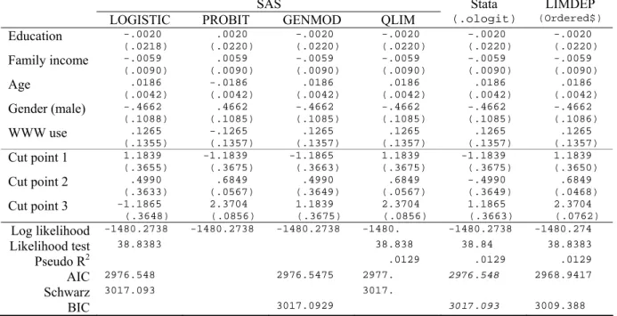
2.4 Ordinal Logit Model in SAS
QLIM, LOGISTIC, and PROBIT procedures estimate ordinal logit and probit models. As
shown in Tables 2.1 and 3.2, PROC QLIM is most recommended. The DIST=LOGISTIC
below fits the ordinal logit egression model using the standard logistic probability distribution.
Stata and PROC QLIM report same goodness-of-fit measures, parameter estimates, and
standard errors.
PROC QLIM DATA=masil.gss_cdvm;
MODEL belief = educate income age male www /DISCRETE (DIST=LOGISTIC);
The QLIM Procedure
Discrete Response Profile of belief
Index Value Frequency Percent 1 0 192 16.35 2 1 134 11.41 3 2 456 38.84 4 3 392 33.39 Model Fit Summary
Number of Endogenous Variables 1 Endogenous Variable belief Number of Observations 1174 Log Likelihood -1480 Maximum Absolute Gradient 5.69774E-6 Number of Iterations 15 Optimization Method Quasi-Newton AIC 2977 Schwarz Criterion 3017 Goodness-of-Fit Measures
Measure Value Formula
Likelihood Ratio (R) 38.838 2 * (LogL - LogL0) Upper Bound of R (U) 2999.4 - 2 * LogL0 Aldrich-Nelson 0.032 R / (R+N) Cragg-Uhler 1 0.0325 1 - exp(-R/N)
Cragg-Uhler 2 0.0353 (1-exp(-R/N)) / (1-exp(-U/N)) Estrella 0.0327 1 - (1-R/U)^(U/N)
Adjusted Estrella 0.0193 1 - ((LogL-K)/LogL0)^(-2/N*LogL0) McFadden's LRI 0.0129 R / U Veall-Zimmermann 0.0446 (R * (U+N)) / (U * (R+N)) McKelvey-Zavoina 0.1019 N = # of observations, K = # of regressors Algorithm converged. Parameter Estimates Standard Approx Parameter DF Estimate Error t Value Pr > |t| Intercept 1 1.183894 0.367498 3.22 0.0013 educate 1 -0.002015 0.022004 -0.09 0.9271 income 1 -0.005921 0.008998 -0.66 0.5105 age 1 0.018646 0.004212 4.43 <.0001 male 1 -0.466195 0.108542 -4.30 <.0001 www 1 0.126483 0.135709 0.93 0.3513
_Limit2 1 0.684929 0.056692 12.08 <.0001 _Limit3 1 2.370441 0.085565 27.70 <.0001
However, Stata and PROC QLIM present cut points in a different way. Unlike Stata, PROC
QLIM estimates the intercept,
2, and
3, assuming
1
0
. The estimated intercept (1.1839) of
PROC QLIM is the same as -
/cut1
in Stata: - (-1.1839). The
_Limit2
above is the deviation of
1
from
2, .6849 =
ˆ
2
ˆ
1=-.4990-(-1.1839);
ˆ
2-.4990 is the value of
/cut2
in Stata (see
Section 5.1). Similarly,
_Limit2
is 2.3704=
ˆ
3
ˆ
1=1.1865-(-1.1839), where 1.1865 is the
value of
/cut3
in Stata. See Long and Freese (2003: 148-149) for discussion on this issue.
PROC LOGISTIC and PROC PROBIT estimate ordinal logit and probit models when a ordinal
dependent variable is specified. The DESCENDING option is used to switch the signs of
coefficients. PROC LOGISTIC conducts the Brant test on the parallel regression assumption,
although the chi-squared 22.64 is slightly larger than 21.94 of
.brant
in Section 5.3 (22.64
versus 21.94). The hypothesis of the proportional odds assumption is rejected (p<.0122).
PROC LOGISTIC DATA = masil.gss_cdvm DESC;
MODEL belief = educate income age male www /LINK=LOGIT;
RUN;
The LOGISTIC Procedure Model Information Data Set MASIL.GSS_CDVM
Response Variable belief belief Number of Response Levels 4
Model cumulative logit Optimization Technique Fisher's scoring Number of Observations Read 1174 Number of Observations Used 1174 Response Profile
Ordered Total Value belief Frequency 1 3 392 2 2 456 3 1 134 4 0 192
Probabilities modeled are cumulated over the lower Ordered Values. Model Convergence Status
Score Test for the Proportional Odds Assumption Chi-Square DF Pr > ChiSq 22.6404 10 0.0122 Model Fit Statistics
Intercept Intercept and Criterion Only Covariates AIC 3005.386 2976.548 SC 3020.590 3017.093 -2 Log L 2999.386 2960.548 Testing Global Null Hypothesis: BETA=0
Test Chi-Square DF Pr > ChiSq Likelihood Ratio 38.8383 5 <.0001 Score 38.2773 5 <.0001 Wald 38.2220 5 <.0001 Analysis of Maximum Likelihood Estimates
Standard Wald
Parameter DF Estimate Error Chi-Square Pr > ChiSq Intercept 3 1 -1.1865 0.3648 10.5771 0.0011 Intercept 2 1 0.4990 0.3633 1.8863 0.1696 Intercept 1 1 1.1839 0.3655 10.4906 0.0012 educate 1 -0.00201 0.0218 0.0085 0.9265 income 1 -0.00592 0.00903 0.4303 0.5119 age 1 0.0186 0.00417 19.9857 <.0001 male 1 -0.4662 0.1088 18.3660 <.0001 www 1 0.1265 0.1355 0.8704 0.3508 Odds Ratio Estimates
Point 95% Wald Effect Estimate Confidence Limits educate 0.998 0.956 1.042 income 0.994 0.977 1.012 age 1.019 1.011 1.027 male 0.627 0.507 0.776 www 1.135 0.870 1.480
Association of Predicted Probabilities and Observed Responses Percent Concordant 57.9 Somers' D 0.168
Percent Discordant 41.1 Gamma 0.169 Percent Tied 0.9 Tau-a 0.117 Pairs 480928 c 0.584
Stata
.ologit
and PROC LOGISTIC produce the same parameter estimates and similar
(slightly different) standard errors. Intercept 1 (1.1839) through 3 (-1.1865) are equivalent to
/cut1
(-1.1839) through
/cut3
(1.1865) but their signs are switched. If you omit DESC, you
will get the same cut points but parameter estimates of regressors will have opposite signs
instead.
PROC GENMOD also fits the ordinal logit model with /DIST=MULTINOMIAl and
/LINK=CLOGIT (or CUMLOGIT). Two options respectively indicate the multinomial
probability distribution and cumulative logit function. This procedure with DESC produces the
same parameter estimates and goodness-of-fit statistics. All cut points have opposite signs and
cut point 1 and 3 are switched. Indeed, it is confusing. The output for parameter estimates is
selectively displayed below.
PROC GENMOD DATA = masil.gss_cdvm DESC;
CLASS belief;
MODEL belief = educate income age male www /DIST=MULTINOMIAL LINK=CLOGIT;
RUN;
The GENMOD Procedure
Analysis Of Maximum Likelihood Parameter Estimates
Standard Wald 95% Confidence Wald
Parameter DF Estimate Error Limits Chi-Square Pr > ChiSq Intercept1 1 -1.1865 0.3663 -1.9044 -0.4687 10.50 0.0012 Intercept2 1 0.4990 0.3649 -0.2162 1.2141 1.87 0.1715 Intercept3 1 1.1839 0.3675 0.4636 1.9042 10.38 0.0013 educate 1 -0.0020 0.0220 -0.0451 0.0411 0.01 0.9271 income 1 -0.0059 0.0090 -0.0236 0.0117 0.43 0.5105 age 1 0.0186 0.0042 0.0104 0.0269 19.59 <.0001 male 1 -0.4662 0.1085 -0.6789 -0.2535 18.45 <.0001 www 1 0.1265 0.1357 -0.1395 0.3925 0.87 0.3513 Scale 0 1.0000 0.0000 1.0000 1.0000
PROC PROBIT produces the same parameter estimates and standard errors with opposite
signs. This command returns the same cut points as those of PROC QLIM except for the sign
of the intercept. PROC QLIM and PROC PROBIT report 1.1839 and -1.1839, respectively.
PROC PROBIT DATA = masil.gss_cdvm;
CLASS belief;
MODEL belief = educate income age male www /DIST=LOGISTIC;
RUN;
The Probit Procedure
Analysis of Maximum Likelihood Parameter Estimates Standard 95% Confidence Chi-
Parameter DF Estimate Error Limits Square Pr > ChiSq Intercept 1 -1.1839 0.3675 -1.9042 -0.4636 10.38 0.0013 Intercept2 1 0.6849 0.0567 0.5738 0.7960 145.97 <.0001 Intercept3 1 2.3704 0.0856 2.2027 2.5381 767.49 <.0001 educate 1 0.0020 0.0220 -0.0411 0.0451 0.01 0.9271 income 1 0.0059 0.0090 -0.0117 0.0236 0.43 0.5105 age 1 -0.0186 0.0042 -0.0269 -0.0104 19.59 <.0001 male 1 0.4662 0.1085 0.2535 0.6789 18.45 <.0001 www 1 -0.1265 0.1357 -0.3925 0.1395 0.87 0.3513
2.5 Ordinal Probit Model in SAS
PROC QLIM by default estimates a probit model. The DIST=NORMAL in the following
procedure can be omitted.
PROC QLIM DATA=masil.gss_cdvm;
MODEL belief = educate income age male www /DISCRETE (DIST=NORMAL);
RUN;
The QLIM Procedure
Discrete Response Profile of belief
Index Value Frequency Percent 1 0 192 16.35 2 1 134 11.41 3 2 456 38.84 4 3 392 33.39 Model Fit Summary
Number of Endogenous Variables 1 Endogenous Variable belief Number of Observations 1174 Log Likelihood -1480 Maximum Absolute Gradient 0.0004222 Number of Iterations 15 Optimization Method Quasi-Newton AIC 2975 Schwarz Criterion 3016 Goodness-of-Fit Measures
Measure Value Formula
Likelihood Ratio (R) 40.13 2 * (LogL - LogL0) Upper Bound of R (U) 2999.4 - 2 * LogL0 Aldrich-Nelson 0.0331 R / (R+N) Cragg-Uhler 1 0.0336 1 - exp(-R/N)
Cragg-Uhler 2 0.0364 (1-exp(-R/N)) / (1-exp(-U/N)) Estrella 0.0338 1 - (1-R/U)^(U/N)
McFadden's LRI 0.0134 R / U Veall-Zimmermann 0.046 (R * (U+N)) / (U * (R+N)) McKelvey-Zavoina 0.0397 N = # of observations, K = # of regressors Algorithm converged. Parameter Estimates Standard Approx Parameter DF Estimate Error t Value Pr > |t| Intercept 1 0.713805 0.218273 3.27 0.0011 educate 1 -0.001519 0.013070 -0.12 0.9075 income 1 -0.002738 0.005371 -0.51 0.6102 age 1 0.010969 0.002475 4.43 <.0001 male 1 -0.290305 0.064630 -4.49 <.0001 www 1 0.064241 0.080919 0.79 0.4273 _Limit2 1 0.395983 0.032090 12.34 <.0001 _Limit3 1 1.433728 0.048873 29.34 <.0001
PROC QLIM and
.oprobit
produce almost the same parameter estimates and standard errors
but present
min a different manner. The intercept .7138 is the value of
/cut1
in Stata with an
opposite sign.
_Limit2
is the deviation of
1from
2: .3960 =
2-
1=-.3178-(-.7138).
Similarly,
_Limit3
is 1.4337 =
3-
1=.7199-(-.7138).
PROC LOGISTIC also estimates the ordinal probit model with /LINK=PROBIT. The test for
the parallel regression assumption reports a large chi-squared of 21.3229 and reject the null
hypothesis (p<.0190). PROC LOGISTIC returns the same parameter estimates but slightly
different standard errors, compared to PROC QLIM and Stata.
PROC LOGISTIC DATA = masil.gss_cdvm DESC;
MODEL belief = educate income age male www /LINK=PROBIT;
RUN;
The LOGISTIC Procedure Model Information Data Set MASIL.GSS_CDVM
Response Variable belief belief Number of Response Levels 4
Model cumulative probit Optimization Technique Fisher's scoring Number of Observations Read 1174 Number of Observations Used 1174 Response Profile