Hybrid inversion method to estimate hydraulic
transmissivity by combining multiple-point
statistics and a direct inversion method
Alessandro Comunian
∗Dipartimento di Scienze della Terra “A.Desio” Università degli Studi di Milano, Milan, Italy
Mauro Giudici
†Dipartimento di Scienze della Terra “A.Desio” Università degli Studi di Milano, Milan, Italy
This is the personal version of the manuscript published on
Mathematical Geosciences,
DOI: 10.1007/s11004-018-9727-0
Abstract
Inversion methods that rely on measurements of the hydraulic headh
cannot capture the fine scale variability of the hydraulic properties of an aquifer. This is particularly true for direct inversion methods, which have the further limitation of providing only deterministic results. On the other hand, stochastic simulation methods can reproduce the fine-scale hetero-geneity but cannot directly incorporate information about the hydraulic gradient. In this work a hybrid approach is proposed to join a direct inver-sion method (the comparison model method, CMM) and multiple-point statistics (MPS), for determination of a hydraulic transmissivity fieldT
from a map of a reference hydraulic headh(ref)
and a prior model of the heterogeneity (a training image). The hybrid approach was tested and compared with pure MPS and pure CMM approaches in a synthetic case study. Also, sensitivity analysis was performed to test the importance of the acceptance thresholdδ, a simulation parameter that allows one to tune the influence ofh(ref)on the final results. The transmissivity fieldsT
obtained using the hybrid approach take into account information coming from the hydraulic gradient while simultaneously reproducing some of the fine scale features provided by the training image. Furthermore, many realizations of T can be obtained thanks to the stochasticity of MPS. Nevertheless, it is not straightforward to exploit the correlation between theT maps provided by the CMM and the prior model introduced by the training image, because the former depends on the boundary conditions and flow settings. Another drawback is the growing number of simulation
∗e-mail: [email protected]; corresponding author †e-mail: [email protected]
parameters introduced when combining two diverse methods. At the same time, this growing complexity opens new possibilities that deserve further investigation.
1
Introduction
In hydrogeology, the problem of determining the hydraulic transmissivity fieldT
of an aquifer is often tackled using inversion methods that rely on information
coming from the hydraulic head h. For this reason, many inversion methods
cannot capture the fine-scale details of the hydraulic heterogeneity, because such
information is filtered out byh(Giudici and Vassena, 2008). This is particularly
true for direct inversion methods, which strongly rely on estimates ofh.
On the other hand, stochastic simulation methods, for example those that rely on some prior models of heterogeneity provided by two-point statistics (a variogram) or multiple-point statistics (a training image), cannot directly
incorporate information coming from measurements ofh.
Many authors have proposed approaches to address these two problems; their efforts were discussed and summarized in a recent review by Linde et al. (2015). Recent trends and the evolution of inverse methods in hydrogeology were also recently discussed by Zhou et al. (2014).
Carrera and Neuman (1986) were among the first to propose a successful in-verse method, based on maximization of a likelihood function, the hypothesis of multi-Gaussianity of the data, and zonation. As a consequence of these assump-tions, that method can hardly reproduce heterogeneity at small wavelengths. de Marsily et al. (1984) proposed the pilot points method (PiPM) to improve the fine-scale variability of the estimated parameter fields. Their method is based on the successive updating of a Kriging field. Some fictitious additional points
(pilot points) are added to the points whereT was obtained with field tests, and
Kriging is applied in an iterative fashion to improve the fit with the observations. The principle of the PiPM was then elaborated by Sahuquillo et al. (1992) and Gómez-Hernández et al. (1997) with the self-calibrated method (SCM). This method explores the advantages of inverse stochastic modeling by providing multiple realizations of the parameter fields under study, conditional to the state observations.
Both the PiPM and SCM rely on a prior model built upon two-point statis-tics. A number of authors have demonstrated the need for new and richer models of heterogeneity, beyond the restrictions of the variogram or multi-Gaussian as-sumption (e.g., Kerrou et al., 2008; Zinn and Harvey, 2003). An alternative to two-point statistics is to draw the prior information from training images, us-ing multiple-point statistics (MPS, Strebelle, 2002; Mariethoz and Caers, 2014). This technique is among the promising tools for development of stochastic in-verse modeling approaches (Zhou et al., 2014).
The works of Lochbühler et al. (2014), Laloy et al. (2016), Li et al. (2012, 2013, 2014), Ronayne et al. (2008), and Alcolea and Renard (2010) describe some recent developments and example applications of MPS within stochastic inversion frameworks. These works range from applications where conditioning data are based on geophysical measurements (Lochbühler et al., 2014), appli-cations focused on data assimilation procedures based on ensemble an Kalman filter (EnKF, Li et al., 2012, 2013, 2014), applications integrating MPS with
dy-namic data using the probability perturbation method in a Bayesian framework (Ronayne et al., 2008), and applications that take into account a connectiv-ity constraint and head measurements with an acceptance/rejection criterion (Alcolea and Renard, 2010).
Notwithstanding this growing number of applications, there is still a need to explore the application of MPS within inversion frameworks; for instance, none of the above-mentioned works ever attempted to exploit the flexibility of MPS by combining it with a direct inverse method. This is done in this work, where MPS is combined with the comparison model method (CMM, Ponzini and Lozej, 1982). Despite the limitations of direct inversion methods (Zhou et al., 2014), the CMM has the advantage of being computationally parsimonious. The proposed hybrid method allows one to (i) include stochasticity in a deterministic inversion method, (ii) integrate MPS data related to the hydraulic head field and (iii) reproduce, at least partially, structures with relatively complex fine-scale structure.
Section 2 briefly recalls the working principles of the CMM and MPS and
describes the workflow of the proposed hybrid inversion approach. It also de-scribes an illustrative case study that will be used to test the proposed approach, and the comparison criteria adopted. The results obtained with a pure CMM,
a pure MPS, and the proposed hybrid approach are reported in Sect.3. Section
4 presents a discussion of the results, while Sect. 5 ends the manuscript with
some concluding remarks.
2
Methods
The hybrid inversion method proposed herein is obtained by combining two techniques: one direct inversion method, i.e., the comparison model method (CMM, Ponzini and Lozej, 1982), and one geostatistical simulation algorithm, i.e., the direct sampling (DS, Mariethoz et al., 2010), which is part of a family of simulation methods based on multiple-point statistics (Guardiano and Srivas-tava, 1993; Strebelle, 2002). Note that, although two particular techniques are combined in this work, the proposed hybrid inversion workflow has a general validity; for example, DS could be replaced by another multiple-point
simu-lation paradigm, for example snesim (Strebelle, 2002) or impala (Straubhaar
et al., 2011), or any other geostatistical simulation technique that can integrate maps of auxiliary variables. DS is selected here due to its flexibility in handling auxiliary information and the possibility of reproducing connected and realistic patterns of heterogeneity.
In the following, the term “pure” is used in opposition to “hybrid” to describe the simulation approaches where either only MPS or only CMM is used.
2.1
Comparison Model Method
The comparison model method (CMM) is a direct inversion method useful for
determination of a hydraulic transmissivity field T given a source term F, a
tentative initial transmissivity field Tk(CM)=0 (the transmissivity of a comparison model, CM), some boundary conditions (BCs), and a reference hydraulic head
Crosta, 1988). The latter is very often interpolated from sparse measurements
of the hydraulic headhover the domain to be characterized.
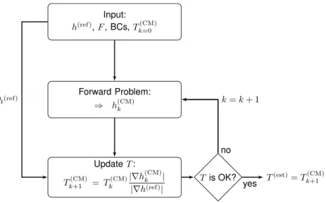
Figure1 illustrates the working principle of the CMM as a flowchart. The
main idea is to update iteratively an initial fieldTk(CM)=0 . At each iteration k, a forward problem (FP) is solved for a CM that shares the same source terms and boundary conditions as the real problem. Using a tentative transmissivity field
Tk(CM), a head field h(CM)k is obtained. The basic hypothesis applied to update
the transmissivity field is that the hydraulic fluxes computed for the CM should
be very close to the fluxes related to h(ref). In other worlds, the update step
can be expressed as
Tk(CM)+1 =Tk(CM)|∇h
(CM)
k |
|∇h(ref)|, (1)
where the hydraulic gradients ∇h can be computed using a finite-difference
scheme in practical applications. In this way,T(CM)is updated iteratively until
a stopping criterion is met. At the end of this procedure,Tk(CM)+1 is taken as the estimatedT field T(est).
The CMM has been successfully applied in a number of case studies (e.g., Vassena et al., 2012; De Filippis et al., 2016), and beyond the field of hydroge-ology (Lesnic, 2010). One of its strengths is computational efficiency, because at each iteration, one only has to solve a FP, and few iterations are needed
to obtain a reliableT(est) in most cases. Another strength is the possibility of
obtaining a transmissivity field representative of the model scale, i.e., of the spacing of the chosen estimation grid.
Among the weaknesses of the CMM is the difficulty in reproducing the
fine-scale details of a T field. This arises from the fact that h(ref) filters out the
fine-scale features of the underlying parameter field T. Therefore, the aim of
this work is to address this weakness by injecting some a priori information using multiple-point statistics simulation (Guardiano and Srivastava, 1993; Strebelle, 2002).
2.2
Direct Sampling Method (DS)
As for other multiple-point simulation paradigms, DS is based on the concept of a training image (TI), which represents a conceptual model of the hetero-geneity and serves as a database of patterns. Here, the working principle of this technique is briefly outlined; More details can be found in Mariethoz et al. (2010).
The aim of DS is to fill the gaps in the spatial variability of a random variable
Z defined only at limited locations in a simulation grid (SG), by sampling the
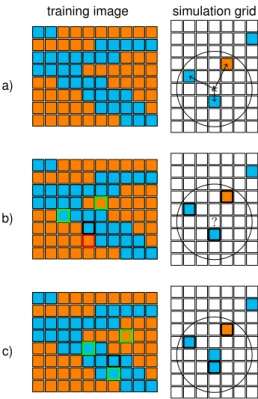
spatial patterns provided by a TI. The sequential DS simulation procedure,
illustrated in Fig. 2, can be summarized as follows:
1. Given a search radius R, randomly select an empty cell at location xin
the SG. The cells of the SG where a value of Z is already defined (or
simulated) and which fall within a radiusR around xare then selected.
Their values, together with their location in the SG with respect tox(the
lag vectorsl1,l2, . . . ), define a data evente={Z(x+l1), Z(x+l2), . . .}
Input: h(ref),F, BCs,T(CM) k=0 Forward Problem: ⇒ h(CM)k UpdateT: Tk(CM)+1 = Tk(CM)|∇h (CM) k | |∇h(ref)| Tis OK? T(est)=T(CM) k+1 no yes k=k+ 1 h(ref)
Figure 1: Flowchart of CMM method
2. The TI is scanned for a data event similar to the data event e defined
in the previous step for the SG. Different measures of similarity can be
adopted to define the distance d between two data events. In the case
of categorical variables, one measure can be based on the number of cells
that present the same value of Z. In the case of continuous variables,
other options are available. Here, theL1-norm is considered.
3. Given a user-defined threshold valueδ, ifd < δthen the similarity between the two data events is “accepted” and the value at the center of the data
event in the TI is pasted at the corresponding grid locationx in the SG
(Fig.2c). Otherwise (Fig.2b), the search continues up to a given stopping
criterion.
These steps are repeated sequentially to fill all the gaps in the SG. In addition,
at the beginning of this procedure, the variableZis normalized in order to work
with dimensionless quantities fordandδ.
The aforementioned procedure can be easily extended to the case of a
mul-tivariate random variableZby providing a multivariate TI, a vector threshold
δ, and a distance for each component ofZ; For example, concerning the choice
of this distance,Zcould be composed of a categorical variable and a continuous
variable. Therefore, one could use a dedicated distance for the categorical
com-ponent of Z and a different distance for its continuous component. Based on
this flexibility, it is easy to imagine a collocated simulation framework, where a bivariate TI is provided while on the SG only one variable is exhaustively known and the other must be simulated. Indeed, this is the setting of the proposed
hybrid method: (a) a bi-variate TI, containing a categorical representation ofT
in terms of facies codes (channel and background) and the corresponding con-tinuous image obtained with the CMM, and (b) a SG where only the concon-tinuous estimate obtained by the CMM is provided, and the categorical representation must be simulated.
training image simulation grid
a)
b) ?
c)
Figure 2: Three basic steps in the DS simulation procedure: a) selection of a random location and a data event in the SG; b) selection of a data event in the TI and compatibility check; c) a compatible data event is found in the TI, and its center value is pasted in the SG
2.3
Hybrid Inversion Method
The proposed hybrid inversion workflow is composed of one preliminary step and one main step. The preliminary step consists in application of the pure CMM approach to create a series of multivariate TIs, one for each iteration
of the CMM. Theh(ref) used for the CMM is obtained by solving a FP with a
training transmissivity fieldT(TI)representing an a priori model of heterogeneity
that is expected to contain the same patterns of heterogeneity as the unknown
T field. T(TI) can be categorical, with a T value provided for each category,
or continuous. In this preliminary step, the pure CMM is run as depicted in
Sect. 2.1 for a given numberK of iterations with given BCs and source term
F. At the end of theKCMM iterations,K transmissivity fieldsTk(TI=1,CM), . . . , Tk(TI=K,CM) are obtained. These fields, combined with T(TI), represent a number
K of bivariate training images(T(TI), Tk(TI=1,CM)), . . . ,(T(TI), Tk(TI=K,CM))that are used in the following step.
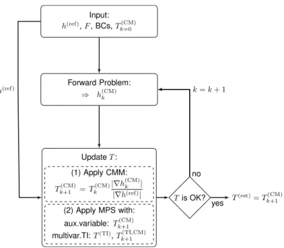
Figure3illustrates the main step. In this step, the h(ref) used in the CMM
steps is not, in general, computed by solving a FP on a fully knownT field, as
it is in the first step. Instead, here h(ref) could be, for example, the result of
an interpolation of some h measurements over an unknown T field that is to
be estimated. Then, the hybrid CMM is applied updatingT in two subsequent
steps. First, Tk(CM)is updated using the information provided by ∇h(CM)k and
∇h(ref), as for the pure CMM, using Eq. (1). Second, the obtained Tk(CM)+1 is
used as a collocated variable to simulate, using DS, a newly updated T. For
the DS simulation, in addition to theTk(CM)+1 used as a collocated variable, the
bivariate TI computed at the previous step for the corresponding k is used,
i.e., (TTI, Tk(TI+1,CM)). As for the pure CMM, this procedure is repeated until a
stopping criterion for the estimatedT is met.
This hybrid inversion framework was implemented using theparflow(Ashby
and Falgout, 1996; Jones and Woodward, 2001; Kollet and Maxwell, 2006;
Maxwell, 2013) and YAGMod (Cattaneo et al., 2015) simulation platforms for
solution of all the FPs, thedeessesoftware (Mariethoz et al., 2010) for the DS
simulation, and Python and its numerical libraries for the CMM and remaining numerical tasks.
2.4
Illustrative Case Study
To illustrate the diverse behaviors of the pure MPS, the pure CMM, and the proposed hybrid approach, the starting point is the TI proposed by Strebelle (2002). A target heterogeneity akin to that TI represents a challenge for all inversion techniques that rely on the two-point correlation paradigm, and would also be a challenge for the pure CMM.
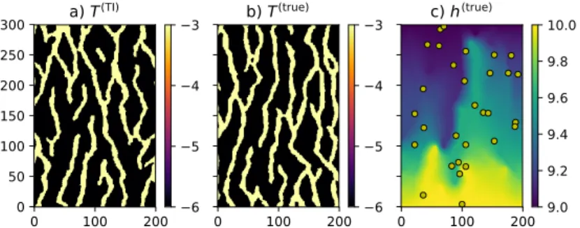
Using the aforementioned TI in a DS simulation framework, two realizations
on a grid of300×200square cells of side25 mwere obtained using thedeesseDS
simulation code (Mariethoz et al., 2010). One of the two realizations was used in the following as a training image itself (T(TI), Fig.4a), while the other was
considered as the (supposed unknown) target transmissivity field that one wishes to reproduce (T(true), Fig.4b). Using average values for sand and shale extracted
from the worldwide hydrolgeological parameters database (http://wwhypda.org,
Input: h(ref),F, BCs,T(CM) k=0 Forward Problem: ⇒ h(CM)k UpdateT: (1) Apply CMM: Tk(CM)+1 =Tk(CM)|∇h (CM) k | |∇h(ref)| (2) Apply MPS with: aux.variable:Tk(CM)+1
multivar.TI:T(TI),T(TI,CM) k+1 Tis OK? T(est)=T(CM) k+1 no yes k=k+ 1 h(ref)
Figure 3: Flowchart for hybrid inversion approach
transmissivity values of 1×10⁻³m2/sand1×10−6m2/swere assigned to the
sand and background shale facies, respectively. In the following, the terminology “low-transmissivity/high-transmissivity” or “background/channel” cells is used interchangeably. In all the simulation settings involving the CMM, the method
was applied considering a null source termFand fixed head boundary conditions
at the borders corresponding to the cell indices j = 1 (h = 10.0 m) and j =
300 (h = 9.0 m), to produce a hydraulic gradient along the main direction of
orientation of the channels, with null flux elsewhere.
Figure 4c shows the head field h(true) obtained from the solution of the
forward problem for the referenceT field; in this map, the yellow dots show the
randomly selected positions of the 30 virtual monitoring points, i.e., the nodes
where it is assumed that h(true) is measured. These data will be compared
with the values computed by solving the forward problem for other estimatedT
fields. Note that these monitoring points are used only for statistics on estimated heads, but not as conditional points for transmissivity or facies.
2.5
Comparison Criteria
The following parameters were used to evaluate the performance of the different
techniques: The proportion of correctly simulated channels (prgt) quantifies
the proportion of simulated channel cells that correspond to a channel in the T(true)grid, while the proportion of incorrectly simulated channels (p
wrg) is the
proportion of simulated channel cells that do not correspond to a channel in the T(true)grid. The Jaccard index (J) somehow summarizes these two parameters
prgt andpwrg. In terms of sets, ifA represents the set of the simulated channel
index is defined as
J = |A∩B|
|A∪B|. (2)
Another parameter considered herein is the proportion of channel facies (p),
that is, the number of channel facies over the total number of grid cells. It is
also useful to examine the probability of connection of two pointsxandy, i.e.,
the probability that two points belong to the same connected component (or
geobody) of the considered domain; this is done using the intrinsic (cint) and
total connectivity (ctot) , as defined by Vassena et al. (2010). These parameters
are related to the hydraulic properties of porous media and therefore provide a synthetic way to summarize them. Here, in particular, the connectivity of the more conductive cells (channel facies) is considered using a four-point scheme. In other words, the connectivity is considered only through the sides of the cells but not through their corners. (See Vassena et al. (2010) for a formal definition, and Renard and Allard (2013) for a comprehensive and recent review about the concept of connectivity and different indicators). Another important morphometric attribute that is useful for comparison of different realizations of a
categorical variable is the number of clusters (N), i.e., the number of connected
components. Here, again, the number of connected components for the channel facies is considered.
All these parameters were computed both on the whole simulation domain and on a subdomain obtained by excluding a boundary frame of size 50 cells on each side. This subdomain is useful to reduce the influence of the boundary conditions on the results of the simulation (an influence that will become evident in the next section in the pure CMM results).
In this work, a synthetic case study is examined, to enable access to a known
transmissivity field T(true) (Fig. 4b). Therefore, in addition to the
aforemen-tioned parameters, the following statistical indicators are adopted to quantify
the errors in the computation of the estimated transmissivity fieldT:
λ = 1 M M X i=1
log10(T(true)(i))−log10(T(est)(i)), (3)
|λ| = 1 M M X i=1 log10(T (true)(i))−log 10(T (est)(i)) , (4) λ2 = 1 M M X i=1
log10(T(true)(i))−log10(T(est)(i))
2
, (5)
whereM is the number of nodes at which the transmissivity is estimated, and
T(true)(i) and T(est)(i) are the transmissivity values at celli, for the reference
and estimated fields, respectively. Note that λ, |λ|, and λ2 are dimensionless
parameters, because they are based on logarithms of transmissivity ratios. In
addition, to quantify the impact that the estimates ofT have on the hydraulic
head h, a root-mean-squared error (RMSE) was computed using the values of
h(true)at the virtual monitoring points (Fig.4c) and the values ofhcomputed
0 100 200 0 50 100 150 200 250 300
a) T
(TI) 0 100 200b) T
(true) 0 100 200c) h
(true) 6 5 4 3 6 5 4 3 9.0 9.2 9.4 9.6 9.8 10.0Figure 4: Decimal logarithm of theT field used as a) training image and as b)
reference. Measurement units are m2/s for T and m for h. Note that, in this
figure and in all the subsequent figures containing maps, values on axes refer to cell indexes
3
Results
In this section, the results obtained using a pure MPS approach, a pure CMM approach, and the proposed hybrid approach are illustrated.
3.1
Pure MPS
To illustrate the differences between the proposed hybrid methodology and a standard approach, the considered reference is an ensemble of 10 pure MPS real-izations performed using different random seeds with standard set of simulation
parameters and the TI presented in Fig. 4a. The parameter sets were selected
according to the guidelines suggested by Meerschman et al. (2013). In particu-lar, a search radius of 124 cells, a maximum number of neighboring cells of 24,
and a threshold δ = 0.05 were selected for scanning the 30 % of the training
image. These same parameter values will be used below in the hybrid approach, apart from relatively small differences required to include a secondary variable. For the moment, in the application of the pure MPS approach, neither hard conditioning data nor soft conditioning data such as auxiliary variable maps were used in the simulations illustrated in this section. The aim here is to eval-uate the default performance of the pure MPS simulation method when trying
to reproduce the referenceT field presented in Fig.4b.
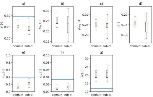
The results of application of the pure MPS approach are illustrated in Fig.5.
A boxplot is drawn for each of the parameters introduced in the previous sec-tions, viz. p,prgt,pwrg,cint,ctot,J, andN, for the full domain and subdomain.
3.2
Pure CMM
This work proposes a hybrid inversion technique that makes use of a direct inversion method and a geostatistical technique. It is therefore useful to briefly present the results that could be obtained using the direct inversion method only, to highlight the improvements introduced when using the proposed hybrid technique.
In a real case study, it is of course not possible to take measurements of the hydraulic head with the same spatial density as the considered discretization grid. Nevertheless, here the results that could be obtained using the pure CMM
domain sub-d. 0.20 0.25 0.30 p [-]
a)
domain sub-d. 0.15 0.20 0.25 0.30 prgt [-]b)
domain sub-d. 0.20 0.25 0.30 pwrg [-]c)
domain sub-d. 0.10 0.15 0.20 J [ -]d)
domain sub-d. 0.0 0.2 0.4 0.6 0.8 1.0 cint [-]e)
domain sub-d. 0.00 0.02 0.04 0.06 0.08 0.10 ctot [-]f)
domain sub-d. 10 15 20 25 30 N [-]g)
Figure 5: Reference parameters for pure MPS simulation, computed on full domain and on subdomain (neglecting an external frame of 50 cells). Horizontal
lines represent parameters computed on the reference field (Fig.4b)
when his known at every point of the discretization grid are briefly outlined.
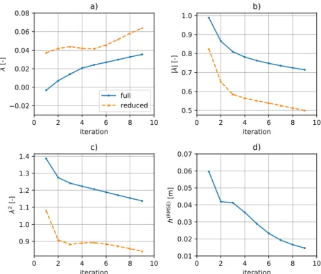
In particular, in Fig.6,λ,|λ|,λ2, and h(RMSE) are plotted against the number
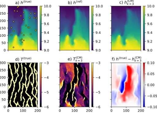
of CMM iterations for the full domain (cyan continuous line) and subdomain (orange dashed line). Figure7shows maps ofh(true),h(ref),h(CM),log10(T(true)),
log10(T(CM)), and(h(true)−h(CM))for the third CMM iteration. This iteration
was chosen to show and discuss the results, becauseλ2attains a local minimum
for the reduced domain, h(RMSE) shows a small variation with respect to the
preceding iteration, and the trend of |λ| becomes less negative for subsequent
iterations.
3.3
Hybrid Approach
As explained in Sect. 2.3, a preliminary step is required before running the
hybrid approach. This step is needed to create the multivariate training images that will be used for the multivariate DS simulations within the workflow of the hybrid approach. These multivariate TIs are obtained by running a pure CMM
approach using ah(ref)computed by solving a FP on theTfield defined by the TI
in Fig.4a. TheT maps created by the pure CMM for each iteration are used in
the multivariate TIs as secondary variable, while the main variable (which is the
same for all iterations) is the TI in Fig.4a. Since within the hybrid approach
the DS is applied with a multivariate TI, a vectorial threshold δ = (δ1, δ2)
is required. The first component (δ1) controls the acceptance threshold for
the categorical variable channel/background, while the second component (δ2)
controls the threshold acceptance for the continuous variable simulated with the CMM.
0 2 4 6 8 10 iteration 0.02 0.00 0.02 0.04 0.06 0.08 [-]
a)
full reduced 0 2 4 6 8 10 iteration 0.5 0.6 0.7 0.8 0.9 1.0 || [-]b)
0 2 4 6 8 10 iteration 0.9 1.0 1.1 1.2 1.3 1.4 2 [-]c)
0 2 4 6 8 10 iteration 0.01 0.02 0.03 0.04 0.05 0.06 0.07 h (R MS E) [m ]d)
Figure 6: Performance of pure CMM in terms ofλ,|λ|,λ2 andh(RMSE) whenh
is known in all cells of the simulation domain. a)-c) present the trends for the full simulation domain (cyan continuous line) and subdomain (orange dashed line)
0
50
100
150
200
250
300
a) h
(true)b) h
(ref)c) h
k = 3(CM)0
100
200
0
50
100
150
200
250
300
d) T
(true)0
100
200
e) T
(CM) k = 30
100
200
f) h
(true)h
(CM) k = 39.0
9.2
9.4
9.6
9.8
10.0
9.0
9.2
9.4
9.6
9.8
10.0
9.0
9.2
9.4
9.6
9.8
10.0
6
5
4
3
6
5
4
3
0.10
0.05
0.00
0.05
0.10
Figure 7: Results of CMM inversion after three iterations: a) truehfield (yellow
dots represent locations used to computeh(RMSE)), b) referencehused as input
for the CMM (in this case h(ref) = h(true)), c) h computed with the T field
estimated with the CMM, d) logarithm of the reference T field, e) logarithm
of the T field estimated with the CMM, f) h(true)−h(CM). Units are m for
Then, always using a trueh(ref), a sensitivity test was performed onδ 2 only.
3.3.1 Trueh
In this test, the hybrid approach was applied usingh(ref)=h(true)as input, i.e.,
anhfield obtained by solving a FP using the trueT (Fig.4b). This setting is of
course far from the real case situation; still, it is useful to verify the performance of the proposed hybrid approach in an ideal case.
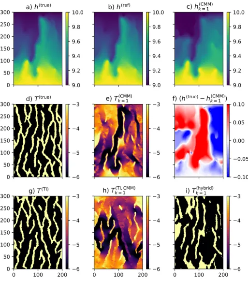
Figure8 shows the same maps presented in Fig.7for the pure CMM, with
three additional maps: g) the binary component of the multivariate TI image
(Fig. 4a), h) the continuous component of the multivariate TI, obtained in the
preliminary step by running the pure CMM, and i) the binary result of the hybrid inversion approach.
A crucial parameter that controls the quality of the DS simulation is the
threshold value δused to accept/reject a given data event (Meerschman et al.,
2013). For this example, δ1 andδ2 were fixed at 0.01 and 0.001, respectively.
The next section presents a brief sensitivity analysis onδ2.
3.3.2 Sensitivity Analysis on the Threshold δ2 for the Secondary Variable
As anticipated in Sect.3.3.1, the acceptance thresholdδplays an important role
in the results of the DS simulations. In this example, the effects of variation of this parameter (δ2) are illustrated for the secondary variable, i.e.,T(CM). A
different value of δ2 corresponds to giving a different weight to the information
provided by h(ref)in the hybrid approach. To illustrate the effects of changing
δ2, the results of the first 10 iterations of the hybrid approach were stacked and
an average value computed and mapped for δ2 = 0.001, δ2 = 0.1, δ2 = 0.2,
and δ2 = 0.5 (Fig. 10). It is also useful to compare the results obtained using
different values of δ2 in quantitative terms. Figures 11 and 12show boxplots
ofN andJ obtained by running 10 simulations with the hybrid approach with
different values of δ2. The first boxplot represents N andJ for the pure MPS
approach, while the others correspond to different k-th iteration steps of the
hybrid approach.
3.4
CPU Time
Table1reports the CPU time required to run the three methods. For the times
related to the pure CMM and the hybrid approach, all the iterations required to obtain an acceptable result (in terms of the aforementioned parameters) are considered. These results were obtained by running the case study on a
work-station equipped with an Intel®CoreTMi7 CPU 860 (2.80 GHzclock frequency)
using one core only. However, all the reported times could be further reduced
because bothparflowanddeessecan be run using multiple cores. Note that,
for the hybrid approach, about 98 % of the CPU time is spent on the MPS sim-ulations, while the remaining 2 % is used for solving the FP and by the Python utility script. Notice also that the MPS iteration performed within the hybrid approach is expected to be slower than the pure MPS, because for the hybrid approach two variables are considered.
0
50
100
150
200
250
300
a) h
(true)b) h
(ref)c) h
k = 1(CMM)0
50
100
150
200
250
300
d) T
(true)e) T
k = 1(CMM)f) (h
(true)h
k = 1(CMM))
0
100
200
0
50
100
150
200
250
300
g) T
(TI)0
100
200
h) T
(TI, CMM) k = 10
100
200
i) T
(hybrid) k = 19.0
9.2
9.4
9.6
9.8
10.0
9.0
9.2
9.4
9.6
9.8
10.0
9.0
9.2
9.4
9.6
9.8
10.0
6
5
4
3
6
5
4
3
0.10
0.05
0.00
0.05
0.10
6
5
4
3
6
5
4
3
6
5
4
3
Figure 8: Results of hybrid approach using h(ref) = h(true) and (δ1, δ2) =
(0.01,0.001), first iteration: from a) to f) see Fig. 7, g) logarithm of T field used as categorical training image h) secondary continuous variable used as
training image, i.e., the logarithm of the T computed using the pure CMM in
the preliminary step, i) result of application of hybrid approach
Table 1: CPU time required by the three methods. The number of iterations is meaningful only for the pure CMM and CMM+MPS, corresponding to the
number of iterations needed to obtain an acceptableT field.
method No. iter. CPU time [sec]
Pure MPS - 58.2
Pure CMM 3 4.3
0.225 0.250 0.275 0.300 p [-]
a) proportions (facies 1)
0.2 0.4 0.6 prgt [-]b) right simulated channels
0.1 0.2
pwrg
[-]
c) wrong simulated channel
0.1 0.2 0.3 cint [-]
d) intrinsic connectivity
0.01 0.02 0.03 ctot [-]e) total connectivity
50 100 N [-]f) number of geobodies
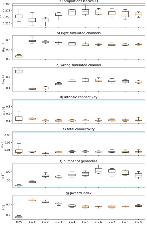
MPS k = 1 k = 2 k = 3 k = 4 k = 5 k = 6 k = 7 k = 8 k = 9 0.2 0.4 J [ -]g) Jaccard index
Figure 9: Comparison of the pure MPS and the hybrid approach. The latter was performed using h(true) as reference h, and (δ1, δ2) = (0.01,0.001). The
first boxplot on the left shows the results of 10 pure MPS simulations, while the
subsequent boxplots, labeled with the index k, represent iterations performed
with the hybrid approach. For each iteration, the results obtained from 10 hybrid simulations using a different random seed were aggregated
0 100 200 0 50 100 150 200 250 300
= 0.001
0 100 200= 0.1
0 100 200= 0.2
0 100 200= 0.5
0.0 0.2 0.4 0.6 0.8 1.0 0.0 0.2 0.4 0.6 0.8 1.0 0.0 0.2 0.4 0.6 0.8 1.0 0.0 0.2 0.4 0.6 0.8 1.0Figure 10: Mean value of simulations (facies codes) obtained over 10 iterations of hybrid approach with different thresholds
0 50 100 N [-]
a)
2= 0.001
0 50 100 N [-]b)
2= 0.1
0 50 100 N [-]c)
2= 0.2
MPS k = 1 k = 2 k = 3 k = 4 k = 5 k = 6 k = 7 k = 8 k = 9 0 50 100 N [-]d)
2= 0.5
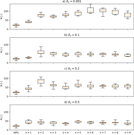
Figure 11: Boxplots of number of geobodies N measured at each iteration for
different values of the thresholdδ. The first boxplot corresponds to a pure MPS
0.1 0.2 0.3 0.4 0.5 0.6 J [-]
a)
2= 0.001
0.1 0.2 0.3 0.4 0.5 0.6 J [-]b)
2= 0.1
0.1 0.2 0.3 0.4 0.5 0.6 J [-]c)
2= 0.2
MPS k = 1 k = 2 k = 3 k = 4 k = 5 k = 6 k = 7 k = 8 k = 9 0.1 0.2 0.3 0.4 0.5 0.6 J [-]d)
2= 0.5
Figure 12: Boxplots of Jaccard index J measured at each iteration for
differ-ent values of the threshold δ. The first boxplot corresponds to a pure MPS
4
Discussion
From the results obtained with the pure MPS approach (Fig. 5), it is clear
that the range of variability of the considered parameters never includes the
target value obtained for T(true). One could probably obtain better results
using other parameter settings. Still, here the aim is not to look for the best parameterization of the MPS, but only to provide a reference case study to be compared with the hybrid approach, where the same parameters are used. Overall, the parameters computed on the subdomain show greater variability, which is probably due to the smaller number of cells on which the parameters are computed.
For the pure CMM approach, the parameters|λ|,λ2, andh(RMSE) show an
almost monotonic decreasing trend, confirming convergence of the maps T(CM)
for increasingk(Fig.6). In particular, the parameterλ2attains a local minimum
at the third iteration for the reduced domain. After this iteration, λ2 for the
whole domain and|λ|show a slowing of their decreasing trend. The bias in the
estimated T field, which is quantified by λ, shows an approximately constant
value up to the sixth iteration, then an increase for the reduced domain, whereas
the increase ofλover the whole domain shows a slight reduction after the third
iteration. h(RMSE) at the third iteration has almost the same value as at the
second iteration, showing a further decrease for subsequent iterations. These
remarks suggest that continuing the iterations to k > 3 does not significantly
improve the results. This is supported by visual inspection of the maps of
Tk(CM) obtained during the diverse iterations; here only the map obtained for
the third iteration is shown (Fig. 7). Only the parameterλshows a discordant
trend, which can be somehow explained by the fact that it is computed by
mixing overestimates and underestimates ofT, and therefore provides less clear
information about the iterative procedure. The maps presented in Fig.7, and
in particular Fig. 7e, show that, in the case when h(ref) = h(true) the CMM
reproduces the envelope of the true T with good detail. Nevertheless, it is
important to note that (i) the provided estimate in not categorical like the target
T, (ii) there are strong differences between the percolating channels, i.e., the
high-transmissivity channels that link the upper and lower part of the domain where the fixed head BCs are applied, and the disconnected channels, and (iii)
noticeable differences in the estimatedT can be observed at the boundaries of
the domain too.
The observations made for the pure CMM approach can be partially ex-tended to the results of the hybrid approach. In this case, the same contrast between percolating channels and disconnected channels observed for the pure
CMM approach in Fig.7e can be observed for the secondary variable of the TI
(Fig. 8h; see, for example, the almost shaded percolating channel that starts
from the lower side of the domain close to the 150th cell). Again, the same
con-trast can be observed betweenT(est) close to the null flux boundary condition
or close to the fixed head ones. All these observations suggest poor correlation between the primary variable and the secondary variable maps. The result of this poor correlation is evident in the final result (Fig.8i), where the fit between
the estimated channels and the true channels (Fig.8d) is satisfactory only in the
center of the domain. Nevertheless, the Jaccard index J (and the parameters
prgt and pwrg) show that, on average, the hybrid method correctly guesses the
around the target value through the iterations, the connectivity indicators (ctot
andcint) remain stable and comparable to the values estimated using the pure
MPS approach. However, the boxplots of these latter indicators show smaller fluctuations, which are probably due to the additional constraints imposed by h(ref)in the hybrid approach. Overall, the number of geobodies is always bigger
for the hybrid approach, indicating that, especially fork >1, the hybrid
simula-tions are more fragmented than the pure MPS simulasimula-tions. Figure 9also shows
that the first couple of iterations are decisive to fix the values of the statistics that have been examined while subsequent iterations introduce relatively small and often nonsystematic variations.
Concerning the sensitivity analysis performed onδ2, the stacks performed
over the iterations clearly illustrate the importance of this parameter (Fig.10).
For small values (0.001< δ2<0.1) the weight given to the information coming
fromh(ref)is strong and there are small differences between the iterations. When
δ2is increased, more freedom is left to the DS algorithm for the simulation of the
categorical facies, and there is greater variability from one iteration to another.
These observations are confirmed, for example, by the variability of J and N
(Figs.11and12). In the case ofN, on average its values are smaller and closer
to the pure MPS results. In other words, when the constraint onh(ref)is looser,
the multivariate MPS produces more realistic channels. On the other hand, in terms ofJ, a stronger constraint onh(ref)(δ
2<0.1) results in better localization
of the channel facies and background facies in the simulation grid.
5
Conclusions
This work represents one of the first attempts to combine multiple-point statis-tics and a direct inversion method (the comparison model method, CMM) into a hybrid inversion approach. The results obtained so far are encouraging. The proposed hybrid approach allows one to address a number of limitations of the
CMM: (i) it allows one to obtain multiple realizations of the estimatedT field
by exploiting the stochasticity of the MPS; (ii) the result can be obtained di-rectly as categorical variables; (iii) in the central part of the simulation domain, a good portion of the facies codes are estimated at the correct locations; (iv) some fine-scale structures can be partially reproduced. At the same time, the hy-brid approach allows one to integrate auxiliary information about the hydraulic heads into multiple-point statistics.
In addition to these advantages, the results highlight a number of limita-tions of the proposed approach. First is the fact that the relalimita-tionship between the primary variable and the secondary variable obtained with the CMM is not straightforward and can be misleading. Indeed, the latter variable is strongly dependent on the hydraulic gradient, and this results in very different responses; See , for example , the strong differences between percolating and disconnected
channels (Fig. 8e, h). For the same reason, the correlation between the facies
codes and the secondary variable computed by the CMM depends on the pres-ence of boundary conditions.
To cope with these nonstationarities in the map of the secondary variable, one could incorporate into the MPS step additional maps representing, for example, the distance from the sides of the domain. A study of this setting deserves further investigation.
The present study suffers from another limitation in that only a setting where h(ref)is fully known at all nodes of the simulation domain has been explored so
far. Therefore, the next steps of this research should investigate the response
of the hybrid approach to an inputh(ref)obtained by interpolation of a limited
number of measurements.
Another interesting result arising from the sensitivity analysis is the rele-vance of the threshold value for the secondary variable: smaller values (below 0.01) provide a good constraint on the observed hydraulic head, but deteriorate the overall properties provided by the first component of the TI. Therefore, for small values of the threshold the simulations appear more fragmented and less connected.
When combining two different tools such as multiple-point statistics and a direct inversion method, the number of simulation parameters grows to become somehow cumbersome. This is particularly true when the multivariate training image has more than two components, or the direct method is applied with a tomographic approach. These remarks should be recalled when generalizing the results of the test case discussed herein: the optimal choice of the parameters of the hybrid approach and of the two basic algorithms is not straightforward. Notwithstanding this growing complexity, the proposed hybrid approach opens new perspectives for inversion of hydraulic parameters of aquifers.
Acknowledgements
The authors thank P. Renard, G. Mariethoz and G. Pirot for the fruitful dis-cussions, and two anonymous reviewers and the editor for their constructive comments, and J. Straubhaar and the University of Neuchâtel for providing the deessesimulation code.
References
Alcolea A, Renard P (2010) Blocking moving window algorithm: Conditioning multiple-point simulations to hydrogeological data. Water Resour Res 46(8),
URLhttp://dx.doi.org/10.1029/2009WR007943
Ashby S, Falgout R (1996) A parallel multigrid preconditioned conjugate gradi-ent algorithm for groundwater flow simulations. Nuclear Science Engineering 124(1):145–159
Carrera J, Neuman SP (1986) Estimation of aquifer parameters under transient and steady state conditions: 1. maximum likelihood method incorporating prior information. Water Resources Research 22(2):199–210, DOI 10.1029/ WR022i002p00199
Cattaneo L, Comunian A, de Filippis G, Giudici M, Vassena C (2015) Modeling groundwater flow in heterogeneous porous media with yagmod. Computation 4(1):2, DOI 10.3390/computation4010002
Comunian A, Renard P (2009) Introducing wwhypda: a world-wide collabora-tive hydrogeological parameters database. Hydrogeology Journal 17(2):481– 489, DOI 10.1007/s10040-008-0387-x
De Filippis G, Giudici M, Margiotta S, Negri S (2016) Conceptualization and characterization of a coastal multi-layered aquifer system in the taranto gulf (southern italy). Environmental Earth Sciences 75(8):686, DOI 10.1007/ s12665-016-5507-7
de Marsily G, Lavedan G, Boucher M, Fasanino G (1984) Interpretation of interference tests in a well field using geostatistical techniques to fit the per-meability distribution in a reservoir model. In: Verly Gea (ed) Geostatistics for natural resources characterization, Proceedings of the NATO Advanced Study Institute, Reidel Publishing Company, Dordrecht, p 831–849
Giudici M, Vassena C (2008) Spectral analysis of the balance equa-tion of ground water hydrology. Transport in Porous Media 72(2):171–
178, DOI 10.1007/s11242-007-9142-3, URL http://dx.doi.org/10.1007/
s11242-007-9142-3
Guardiano FB, Srivastava RM (1993) Multivariate geostatistics: Beyond bivari-ate moments. In: Soares A (ed) Geostatistics: Troia ’92, Kluwer, Dordrecht, The Netherlands, vol 1, pp 133–144
Gómez-Hernández JJ, Sahuquillo A, Capilla JE (1997) Stochastic simulation of transmissivity fields conditional to both transmissivity and piezometric data—i. theory. Journal of Hydrology 203(1):162 – 174, DOI http://dx.doi. org/10.1016/S0022-1694(97)00098-X
Jones JE, Woodward CS (2001) Newton–krylov-multigrid solvers for large-scale, highly heterogeneous, variably saturated flow problems. Advances in Water
Resources 24(7):763 – 774, DOI 10.1016/S0309-1708(00)00075-0, URLhttp:
//www.sciencedirect.com/science/article/pii/S0309170800000750
Kerrou J, Renard P, Franssen HJH, Lunati I (2008) Issues in characterizing het-erogeneity and connectivity in non-multigaussian media. Advances in Water Resources 31(1):147 – 159, DOI http://dx.doi.org/10.1016/j.advwatres.2007. 07.002
Kollet J, Maxwell R (2006) Integrated surface-groundwater flow modeling: a free-surface overland flow boundary condition in a parallel groundwater flow model. Advances in Water Resources 29(7):945–958
Laloy E, Linde N, Jacques D, Mariethoz G (2016) Merging parallel tempering with sequential geostatistical resampling for improved posterior exploration of high-dimensional subsurface categorical fields. Advances in Water Resources 90:57 – 69, DOI http://dx.doi.org/10.1016/j.advwatres.2016.02.008
Lesnic D (2010) The comparison model method for determining the flexural rigidity of a beam. Journal of Inverse and Ill-posed Problems 18(5):577–590, DOI 10.1515/jiip.2010.026
Li L, Zhou H, Hendricks Franssen HJ, Gómez-Hernández JJ (2012) Groundwater flow inverse modeling in non-multigaussian media: performance assessment of the normal-score ensemble kalman filter. Hydrology and Earth System Sci-ences 16(2):573–590, DOI 10.5194/hess-16-573-2012
Li L, Srinivasan S, Zhou H, Gómez-Hernández J (2013) A pilot point guided pattern matching approach to integrate dynamic data into geological model-ing. Advances in Water Resources 62, Part A:125 – 138, DOI http://dx.doi. org/10.1016/j.advwatres.2013.10.008
Li L, Srinivasan S, Zhou H, Gomez-Hernandez J (2014) Simultaneous estimation of geologic and reservoir state variables within an ensemble-based multiple-point statistic framework. Mathematical Geosciences 46(5):597–623, DOI 10.1007/s11004-013-9504-z
Linde N, Renard P, Mukerji T, Caers J (2015) Geological realism in hydrogeolog-ical and geophyshydrogeolog-ical inverse modeling: A review. Advances in Water Resources 86, Part A:86 – 101, DOI http://dx.doi.org/10.1016/j.advwatres.2015.09.019 Lochbühler T, Pirot G, Straubhaar J, Linde N (2014) Conditioning of multiple-point statistics facies simulations to tomographic images. Mathematical Geo-sciences 46(5):625–645, DOI 10.1007/s11004-013-9484-z
Mariethoz G, Caers J (2014) Multiple-point Geostatistics: Stochastic Modeling with Training Images. Wiley, 376 pages
Mariethoz G, Renard P, Straubhaar J (2010) The direct sampling method to perform multiple-point geostatistical simulations. Water Resour Res 46(11):W11,536, DOI 10.1029/2008WR007621
Maxwell RM (2013) A terrain-following grid transform and
precondi-tioner for parallel, large-scale, integrated hydrologic modeling.
Ad-vances in Water Resources 53:109 – 117, DOI https://doi.org/10.1016/
j.advwatres.2012.10.001, URL http://www.sciencedirect.com/science/
article/pii/S0309170812002564
Meerschman E, Pirot G, Mariethoz G, Straubhaar J, Meirvenne MV, Renard P (2013) A practical guide to performing multiple-point statistical simulations with the direct sampling algorithm. Computers & Geosciences 52(0):307 – 324, DOI 10.1016/j.cageo.2012.09.019
Ponzini G, Crosta G (1988) The comparison model method: A new arithmetic approach to the discrete inverse problem of groundwater hydrology. Transport in Porous Media 3(4):415–436, DOI 10.1007/BF00233178
Ponzini G, Lozej A (1982) Identification of aquifer transmissivities: The com-parison model method. Water Resources Research 18(3):597–622, DOI 10.1029/WR018i003p00597
Renard P, Allard D (2013) Connectivity metrics for subsurface flow and trans-port. Advances in Water Resources 51(0):168 – 196, DOI 10.1016/j.advwatres. 2011.12.001
Ronayne MJ, Gorelick SM, Caers J (2008) Identifying discrete geologic structures that produce anomalous hydraulic response: An inverse mod-eling approach. Water Resources Research 44(8):n/a–n/a, DOI 10.1029/ 2007WR006635, w08426
Sahuquillo A, Capilla J, Gómez-Hernández J, Andreu J (1992) Conditional sim-ulation of transmissivity fields honoring piezometric data. Hydraulic engineer-ing software IV, Fluid flow modelengineer-ing 2:201–214
Scarascia S, Ponzini G (1972) An approximate solution of the inverse problem in hydraulics. L’Energia Elettrica 49:518–531
Straubhaar J, Renard P, Mariethoz G, Froidevaux R, Besson O (2011) An im-proved parallel multiple-point algorithm using a list approach. Mathematical Geosciences 43(3):305–328, DOI 10.1007/s11004-011-9328-7
Strebelle S (2002) Conditional simulation of complex geological structures us-ing multiple-point statistics. Mathematical Geology 34:1–21, DOI 10.1023/A: 1014009426274
Vassena C, Cattaneo L, Giudici M (2010) Assessment of the role of facies heterogeneity at the fine scale by numerical transport experiments and connectivity indicators. Hydrogeology Journal 18(3):651–668, DOI 10.1007/ s10040-009-0523-2
Vassena C, Rienzner M, Ponzini G, Giudici M, Gandolfi C, Durante C, Agostani D (2012) Modeling water resources of a highly irrigated alluvial plain (italy): calibrating soil and groundwater models. Hydrogeology Journal 20(3):449– 467, DOI 10.1007/s10040-011-0822-2
Zhou H, Gómez-Hernández JJ, Li L (2014) Inverse methods in hydrogeology: Evolution and recent trends. Advances in Water Resources 63(0):22 – 37, DOI http://dx.doi.org/10.1016/j.advwatres.2013.10.014
Zinn B, Harvey CF (2003) When good statistical models of aquifer heterogeneity go bad: A comparison of flow, dispersion, and mass transfer in connected and multivariate gaussian hydraulic conductivity fields. Water Resour Res 39(3)