http://researchcommons.waikato.ac.nz/
Research Commons at the University of Waikato
Copyright Statement:
The digital copy of this thesis is protected by the Copyright Act 1994 (New Zealand). The thesis may be consulted by you, provided you comply with the provisions of the Act and the following conditions of use:
Any use you make of these documents or images must be for research or private study purposes only, and you may not make them available to any other person.
Authors control the copyright of their thesis. You will recognise the author’s right to be identified as the author of the thesis, and due acknowledgement will be made to the author where appropriate.
You will obtain the author’s permission before publishing any material from the thesis.
Surrogate-Assisted
Evolutionary Algorithms for
Wind Farm Layout Optimisation
Problem
A thesis
submitted in partial fulfillment of the requirements for the degree
of
Master of Science (Research)
at
The University of Waikato
by
Chen Zheng
Abstract
Due to the increasing need for computationally expensive optimisation in many real-world applications, surrogate-assisted evolutionary algorithms have attracted growing attention. In the literature, surrogate-assisted evolutionary approaches have been successful in highly computational expensive optimisation problems. However, surrogates have not been used with the Wind Farm Layout Optimisation Problem (WFLOP) before.
In this work, an evolutionary approach using surrogate modelling techniques to reduce the computational cost of the WFLOP is studied. The WFLOP mainly focuses on finding the optimal geographical place-ment of wind turbines within a wind farm in order to maximise power generation. But evaluating wind farm layout is very computationally expensive. The purpose of using surrogates is to approximate the real evaluation function of an evolutionary algorithm, but the surrogates can be computed more efficiently. The aim of this study is try to discover whether the surrogate-assisted evolutionary approach is effective on the WFLOP or not.
An analytical wake model from the literture is used to calculate the velocity deficits in the downstream generated by individual turbines. A set of initial offline experiments was conducted based on a dataset of wind farm layouts sampled from the space of all layouts, using biased random walk. These experiments were designed to discover which fea-tures lead to construction of an accurate surrogate model. According to the results of these experiments, polar coordinates (sorted accord-ing to distance) as features are selected for learnaccord-ing. A multilayer
per-tion in conjuncper-tion with an (µ, λ) evolutionary strategy. Two previously presented BlockCopy operators are used in the evolutionary strategy. The surrogate models are managed using a modified version of the Pre-selection strategy and the Best strategy.
Our evaluation used four benchmark wind farm scenarios with di-mensionality ranging from 200 to 1420 dimensions. The evaluation re-sults show that our preliminary MLP and M5P surrogate models did not improve the optimisation results over traditional evolutionary strategies due to scalability issues. The scalability is a known weakness of many surrogate-assisted evolutionary approaches for the reason that most of them are designed for low-dimensionality problems. However, the re-search should continue on this topic because of its importance to renew-able energy.
Acknowledgements
First of all, I would like to express my deepest appreciation and gratitude to my supervisor Dr. Michael Mayo for his expert guidance, understand-ing and encouragement throughout my study and research. He read my numerous revisions and he was always available for my questions. With-out his incredible patience and full support, the completion of this study would not have been possible. It is a great honour to work under his supervision.
Next I would like to thank my parents for their love and support over the years. They have always been there for me and I am thankful for everything they have helped me achieve.
I am also grateful to all the fellow graduate students in the Machine Learning Lab at the Department of Computer Science, the University of Waikato. Especially a thank you to my friend and class fellow Bingyuan Liu for always listening and giving me words of encouragement.
Last but not least, I am thankful to all my friends for helping me survive all the stress from this year. I have no valuable words to express my thanks, but my heart is still full of the favours received from every person.
Contents
1 Introduction 1
2 Wind Farm Layout Optimisation Problem 5
2.1 Wind Farm Layout Example . . . 5
2.2 Wind Farm Wake Effect . . . 7
2.2.1 Wind Turbine Characteristics . . . 7
2.2.2 Surface Roughness . . . 10
2.2.3 Wind Modelling . . . 11
2.2.4 Wake Effect Modelling . . . 13
2.3 Wind Turbine Energy Output . . . 18
2.4 WFLOP Objective Functions . . . 19
2.5 Wind Farm Design Tools . . . 22
2.6 Variants of the WFLOP . . . 24
2.7 Computational Complexity of WFLOP . . . 26
3 Evolutionary Algorithms 29 3.1 Genetic Algorithms . . . 30
3.2 Evolutionary Strategies . . . 31
3.3 Evolutionary Strategies with Elitism . . . 33
3.4 Selection, Mutate and Crossover . . . 34
3.5 Crossover vs. Mutation . . . 35
3.7 Evolutionary Algorithm Applications for WFLOP . . . 38
4 BlockCopy Operators for the WFLOP 43 4.1 BlockCopy Mutation Operator . . . 44
4.2 BlockCopy Crossover Operator . . . 46
5 Surrogate-Assisted Evolutionary Optimisation 49 5.1 Overview . . . 49
5.2 Surrogate Modelling Techniques . . . 51
5.2.1 Quadratic Response Surface Model . . . 52
5.2.2 Kriging Model . . . 55
5.2.3 Artificial Neural Networks . . . 57
5.2.4 Discussion of Different Surrogate Models . . . 61
5.3 Scalability Issues of Surrogate-assisted EAs . . . 62
5.4 The Management of Fitness Approximation in EA . . . 63
5.4.1 A Brief Review on Managing Surrogates . . . 63
5.4.2 Pre-Selection Surrogate Management Strategy . . . 64
5.4.3 Best Surrogate Management Strategy . . . 65
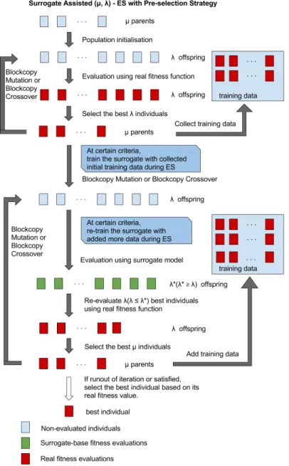
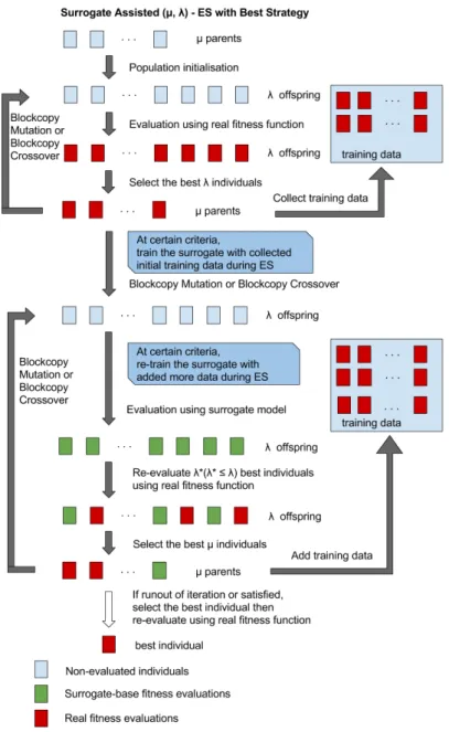
5.4.4 Modified Pre-Selection and Best Surrogate Manage-ment Strategy . . . 66
6 Initial Experiments: Comparison of Different Approximation Models 71 6.1 Approximation Accuracy Measurements . . . 71
6.2 Initial Offline Experiment Data Description . . . 73
6.3 Initial Offline Experiment Setup . . . 75
6.4 Initial Offline Experiment Results . . . 77
7 Evaluation and Results 79 7.1 Wind Farm Scenarios . . . 79
Contents
7.2 Objective Function . . . 81
7.3 Evaluation Setup . . . 83
7.4 Evaluation Results . . . 84
7.4.1 Wind Farm Scenario Kusiak & Song 1 [54] . . . 85
7.4.2 Wind Farm Scenario Kusiak & Song 2 [54] . . . 93
7.4.3 Wind Farm Scenario 2014 Comp 1 [105] . . . 101
7.4.4 Wind Farm Scenario 2014 Comp 3 [105] . . . 109
7.5 Summary of Evaluation Results . . . 117
8 Conclusions 119
List of Figures
2.1 Aerial View of Lillgrund Windfarm [91]. The Lillgrund Wind-farm is located off the coast of Copenhagen in Denmark. . . 6 2.2 Layout of the Middelgrunden offshore wind farm [28]. (a)
ac-tual layout, (b) symmetrically optimised layout, (c) randomly optimised. . . 7 2.3 Simple drawing the rotor and blades of a wind turbine from
a front point of view (left) and a side point of view (right), respectively [36]. . . 8 2.4 Power curve (black line) and thrust coefficient curve (grey
line) of the turbine Vestas V63 [89, 98]. . . 9 2.5 Example of the distance between turbines in both prevailing
wind direction and the direction perpendicular to the prevail-ing wind. There are five turbines each column and the pre-vailing wind blows from left to right. . . 10 2.6 An example of a wind rose diagram, showing statistics of wind
speed and direction throughout the year [4]. This is a wind rose with 16 sectors whereas the center of each sector indi-cates at a given location (i.e a wind farm site). The length of each colour-coded "spoke" around the circle illustrates the relative wind speed in the pointed direction. . . 12 2.7 Wind farm boundary and the definition of the wind speed
di-rection [54]. The two arrows indicate that the wind might come from both both directions. The length of each colour-coded "spoke" around the circle illustrates the relative wind speed in the pointed direction. . . 14 2.8 Schemetic representation of the wake effect. . . 15
2.9 Schemetic representation of multiple wake affecting a position. 15
3.1 Example of Crossover and Mutate Operations. . . 35
3.2 A cube in space formed by two three-dimention vectors (black circles). The space inside the cube represents all possible re-sults produced by crossovering the two vectors. The outer space represents the possible results by mutating the two vec-tors. . . 37
4.1 Illustration of the BlockCopy Mutation Operation. In this ex-ample, blockB2 is chosen for mutation and copied to the po-sition occupied byB6. . . 45
4.2 Illustration of the BlockCopy Crossover Operation. In this ex-ample, block B2 from parent B is chosen is chosen to be re-placed by blockA2 from parentA. . . 46
5.1 Tradeoffs between computational cost and accuracy among different levels of fitness evaluations [9]. . . 50
5.2 Building Surrogate Models via Offline experiments. . . 52
5.3 One node of MLP: an artificial neuron. . . 58
5.4 Architecture of a multilayer perceptron network. . . 59
5.5 Pre-selection Surrogate Management Strategy [46]. . . 65
5.6 Best Surrogate Management Strategy [46]. . . 66
5.7 Collect and prepare wind farm layout data. The layout data consists of raw Cartessian coordinates (xi, Yi) of the wind tur-bines. Then they are converted into polar coordinates (di, θi). At the end the polar coordinates are sorted according to the distancesdbetween the turbines and the zero point. . . 68
5.8 Surrogate Assisted (µ, λ) - ES Using Pre-selection Strategy Strategy with Surrogate-Retraining. . . 69
5.9 Surrogate Assisted (µ, λ) - ES Using Best Strategy Strategy with Surrogate-Retraining. . . 70
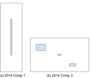
7.1 Obstacles in scenario Comp 1 and Comp 3. Layouts are not shown to scale. . . 80
List of Figures
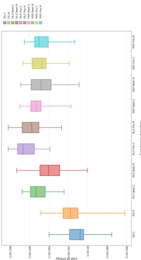
7.2 Wind rose used in each scenario. These wind rose diagrams are not shown to scale. . . 81 7.3 Cost of best layouts found by different evolutionary algorithms
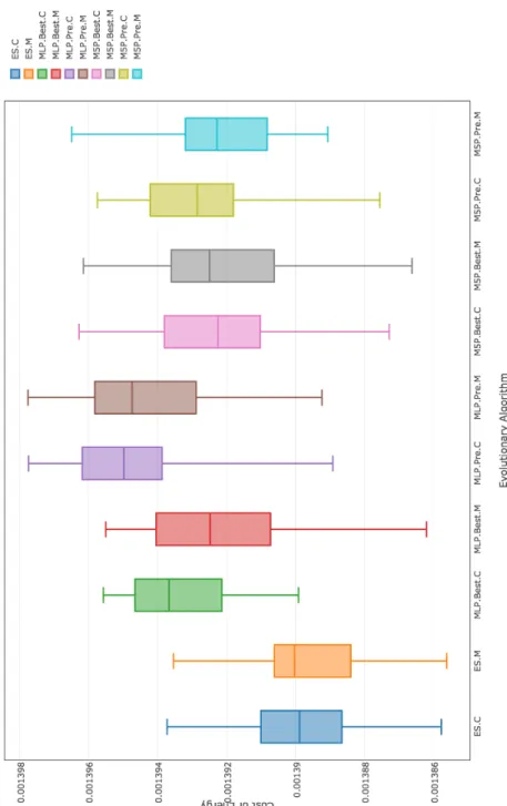
(see Table 7.3) using (6,12) population configuration on the Kusiak & Song 1 [54] wind farm scenario. . . 87 7.4 Cost of best layouts found by different evolutionary algorithms
(see Table 7.3) using (10,20) population configuration on the Kusiak & Song 1 [54] wind farm scenario. . . 88 7.5 Cost of best layouts found by different evolutionary algorithms
(see Table 7.3) using (20,40) population configuration on the Kusiak & Song 1 [54] wind farm scenario. . . 89 7.6 Convergence history of the best layouts found by different
evolutionary algorithms (see Table 7.3) using (6,12) popula-tion configurapopula-tion on the Kusiak & Song 1 [54] wind farm sce-nario. . . 90 7.7 Convergence history of the best layouts found by different
evolutionary algorithms (see Table 7.3) using (10,20) popu-lation configuration on the Kusiak & Song 1 [54] wind farm scenario. . . 91 7.8 Convergence history of the best layouts found by different
evolutionary algorithms (see Table 7.3) using (20,40) popu-lation configuration on the Kusiak & Song 1 [54] wind farm scenario. . . 92 7.9 Cost of best layouts found by different evolutionary algorithms
(see Table 7.3) using (6,12) population configuration on the Kusiak & Song 2 [54] wind farm scenario. . . 95 7.10 Cost of best layouts found by different evolutionary algorithms
(see Table 7.3) using (10,20) population configuration on the Kusiak & Song 2 [54] wind farm scenario. . . 96 7.11 Cost of best layouts found by different evolutionary algorithms
(see Table 7.3) using (20,40) population configuration on the Kusiak & Song 2 [54] wind farm scenario. . . 97
7.12 Convergence history of the best layouts found by different evolutionary algorithms (see Table 7.3) using (6,12) popula-tion configurapopula-tion on the Kusiak & Song 2 [54] wind farm sce-nario. . . 98 7.13 Convergence history of the best layouts found by different
evolutionary algorithms (see Table 7.3) using (10,20) popu-lation configuration on the Kusiak & Song 2 [54] wind farm scenario. . . 99 7.14 Convergence history of the best layouts found by different
evolutionary algorithms (see Table 7.3) using (20,40) popu-lation configuration on the Kusiak & Song 2 [54] wind farm scenario. . . 100 7.15 Cost of best layouts found by different evolutionary algorithms
(see Table 7.3) using (6,12) population configuration on the 2014 Wind Farm Layout Optimisation Comp 1 [105] wind farm scenario. Please note thatµ= 10−6. . . 103 7.16 Cost of best layouts found by different evolutionary algorithms
(see Table 7.3) using (10,20) population configuration on the 2014 Wind Farm Layout Optimisation Comp 1 [105] wind farm scenario. Please note thatµ= 10−6. . . . . 104
7.17 Cost of best layouts found by different evolutionary algorithms (see Table 7.3) using (20,40) population configuration on the 2014 Wind Farm Layout Optimisation Comp 1 [105] wind farm scenario. Please note thatµ= 10−6. . . . . 105
7.18 Convergence history of the best layouts found by different evolutionary algorithms (see Table 7.3) using (6,12) popula-tion configurapopula-tion on the 2014 Wind Farm Layout Optimi-sation Comp 1 [105] wind farm scenario. Please note that
µ= 10−6. . . 106 7.19 Convergence history of the best layouts found by different
evolutionary algorithms (see Table 7.3) using (10,20) popu-lation configuration on the 2014 Wind Farm Layout Optimi-sation Comp 1 [105] wind farm scenario. Please note that
List of Figures
7.20 Convergence history of the best layouts found by different evolutionary algorithms (see Table 7.3) using (20,40) popu-lation configuration on the 2014 Wind Farm Layout Optimi-sation Comp 1 [105] wind farm scenario. Please note that
µ= 10−6. . . . 108
7.21 Cost of best layouts found by different evolutionary algorithms (see Table 7.3) using (6,12) population configuration on the 2014 Wind Farm Layout Optimisation Comp 3 [105] wind farm scenario. . . 111 7.22 Cost of best layouts found by different evolutionary algorithms
(see Table 7.3) using (10,20) population configuration on the 2014 Wind Farm Layout Optimisation Comp 3 [105] wind farm scenario. . . 112 7.23 Cost of best layouts found by different evolutionary algorithms
(see Table 7.3) using (20,40) population configuration on the 2014 Wind Farm Layout Optimisation Comp 3 [105] wind farm scenario. . . 113 7.24 Convergence history of the best layouts found by different
evolutionary algorithms (see Table 7.3) using (6,12) popula-tion configurapopula-tion on the 2014 Wind Farm Layout Optimisa-tion Comp 3 [105] wind farm scenario. . . 114 7.25 Convergence history of the best layouts found by different
evolutionary algorithms (see Table 7.3) using (10,20) popula-tion configurapopula-tion on the 2014 Wind Farm Layout Optimisa-tion Comp 3 [105] wind farm scenario. . . 115 7.26 Convergence history of the best layouts found by different
evolutionary algorithms (see Table 7.3) using (20,40) popula-tion configurapopula-tion on the 2014 Wind Farm Layout Optimisa-tion Comp 3 [105] wind farm scenario. . . 116
List of Tables
2.1 The characteristics of a Wind Turbine. . . 8 2.2 Typical Surface Roughness Lengthes [28]. . . 11
3.1 Common terms used in evolutionary computation. . . 30
5.1 The dimension of optimisation problems reviewed in Section 5.2. 63
6.1 The number of turbines and number of attributes for each sce-nario after each filter is applied. . . 75 6.2 Options for the MLP classifier used in our initial offline
experi-ments. . . 76 6.3 Options for the M5P classifier used in our initial offline
experi-ments. . . 77 6.4 Comparison of correlation coefficient (first line in each cell)
and root relative squared error (second line in each cell) on datasets for wind farm scenario Kusiak & Song 1 [54]. . . 78 6.5 Comparison of correlation coefficient (first line in each cell)
and root relative squared error (second line in each cell) on datasets for wind farm scenario Kusiak & Song 2 [54]. . . 78 6.6 Comparison of (first line in each cell) and root relative squared
error (second line in each cell) on datasets for wind farm sce-nario 2014 Comp 1 [105]. . . 78 6.7 Comparison of (first line in each cell) and root relative squared
error (second line in each cell) on datasets for wind farm sce-nario 2014 Comp 3 [105]. . . 78
7.1 Wind Scenario dimensions, number of turbines, number of blocks and k parameter. . . 81 7.2 The discreption of different evolutionary algorithms. . . 83 7.3 The discreption of different evolutionary algorithms. . . 84 7.4 The average elapsed time of thirty runs of each algorithm
un-der three different population configurations for wind farm sce-nario Kusiak & Song 1 [54]. The unit is milliseconds. . . 86 7.5 The average elapsed time of thirty runs of each algorithm
un-der three different population configurations for wind farm sce-nario Kusiak & Song 2 [54]. The unit is milliseconds. . . 94 7.6 The average elapsed time of thirty runs of each algorithm
un-der three different population configurations for wind farm sce-nario 2014 Wind Farm Layout Optimisation Comp 1 [105]. The unit is milliseconds. . . 102 7.7 The average elapsed time of thirty runs of each algorithm
un-der three different population configurations for wind farm sce-nario 2014 Wind Farm Layout Optimisation Comp 3 [105]. The unit is milliseconds. . . 110
Chapter 1
Introduction
Wind power is becoming increasingly more important around the world along with the rapid development of the global economy. The Global Wind Energy Council (GWEC) reports that globally wind power produc-tion reached 433 gigawatts (GW) by the end of 2015, a cumulative 17% increase. Furthermore, GWEC predicts that by the end of 2030, there will be about 2,000 GW of wind power spinning around the world [27]. It is clear that wind power is now a mainstream source of renewable en-ergy supply and will play a leading role in the future. The wind industry is interested in using technical innovation to drive costs down, improve project reliability and predictability, and make it easier to integrate wind power into the main power grid.
It is obvious that wind farm developers desire a high profit wind farm. In the real world, there is a trade off between two conflicting opposed economical factors: cost of construction and maintenance, and the profit of selling generated electricity. In order to reduce cost and increase profit, wind farm designers are moving towards larger sized farms, more turbines, and other advanced capabilities. However, installing significant numbers of turbines close together causes them to interfere with each other due to the wake effects. The wake effect cases the downstream wind speed to reduce which leads to a considerable loss the power pro-duction, and thus a decrease in profit.
Finding high quality wind farm layout solutions probably will signifi-cantly increase the profit for the wind farm developers. The Wind Farm Layout Optimisation Problem (WFLOP) focuses on finding the optimal turbine positions on a wind farm (wind farm layout) to gain maximum power output. Normally, the WFLOP are conveniently solved using sim-plified rules that lead to rectilinear layouts, where turbines are often organised in identical rows that are separated by an unnecessarily large distance [89]. Recently, a few studies have shown that irregular and nonuniform layouts (see Figure 2.2) can produce more energy than reg-ular grid layouts [54, 88, 93].
In the literature, the related work on this topic are very limited and most of them has been carried out by the wind engineering and renew-able energy communities. There are only a few works has been done by the operations researchers and meta-heuristic algorithms researchers. One reason this problem has been disregarded by the research commu-nity is the computational complexity. For example, even in the case of a simplified single objective function (maximising the wind farm energy output), one wind farm layout evaluation can take minutes, hours, or even days. Due to the high computational complexity, research on the WFLOP are also motivated to reduce the computational cost.
Furthermore, this particular problem requires the researcher to have certain specialist knowledge about how wind model (see Section 2.2.3) and wake model (see Section 2.2.4) are formulated. Additionally, it is difficult to obtain industrial data about the problem instances, which is generally kept private by the wind farm developers [89].
Population-based meta-heuristic approaches such as genetic algo-rithms have found successful in optimisation problems such as portfo-lio selection problems [84], and knapsack problems [82], among many others. However, the WFLOP is generally high-dimensional and compu-tational expensive. Thus it is not practical to apply meta-heuristic ap-proaches to solve the WFLOP since a relatively large number of real fit-ness evaluations are required to obtain a near optimal solution.
On the other hand, surrogate-assisted meta-heuristic optimisation approaches have been shown promising performance in terms of reduc-ing computational cost in many real world expensive optimisation prob-lems [94, 81, 1, 2, 35, 6]. The main idea is to use computationally cheap models, known as surrogates, for approximating the expensive fitness function in evolutionary approaches. However, the surrogates have not been used with the WFLOP before. There is a potential improvement by using meta-heuristic optimisation techniques in conjunction with ma-chine learning algorithms such as decision trees, linear models and artifi-cial neural networks. Additionally, in the literature the maximum dimen-sion of optimisation problem solved by surrogate-assisted evolutionary approach is only 50 [64]. It is also interesting to discovery the perfor-mance of surrogate-assisted meta-heuristic optimisation approaches on four benchmark wind farm scenarios with dimensionality ranging from 200 to 1420 dimensions.
This work focuses on the WFLOP. The main research objective is to develop an approach that can obtain near optimum solutions at a reduced computational cost for practical purposes. This work evaluated several sophisticated evolutionary algorithms using surrogates along with few standard evolutionary algorithms. The choice of surrogate to use is based on a set initial offline experiments on benchmark wind farm scenarios. These experiments also discovered which features lead to the construc-tion of an accurate surrogate model. The previously proposed highly ef-ficient BlockCopy Mutation and Crossover operators [73] are employed to generate offsprings (see Chapter 4). In the evaluation, I compared the final results obtained by different evolutionary algorithms using differ-ent BlockCopy operators with differdiffer-ent surrogate models and surrogate management techniques on four benchmark scenarios from the literature [54, 105].
The rest of this thesis is organised as follows. The background of the wind farm layout optimisation problem is given in Chapter 2. Chap-ter 3 reviews several population-based meta-heuristic algorithms from the literature and a few of their applications for the WFLOP. In
Chap-ter 5, the popular surrogate modelling techniques are briefly described, furthermore, two surrogate model management strategies are explained along with our modification to them. In Chapter 4, the efficient Block-Copy Mutate and Crossover operators previously proposed by [73] are explained. The setup and results of a set of initial offline experiment are shown in Chapter 6. The performance of the surrogate-assisted evo-lutionary strategy using our chosen surrogate models with the modified surrogate management strategies are evaluated on four benchmark wind farm scenarios and compared with that of the evolutionary strategy with-out surrogates in Chapter 7. A brief description of the scenarios and the real fitness function is also included. Finally, Chapter 8 concludes this thesis with a summary and some ideas for future work.
Chapter 2
Wind Farm Layout Optimisation
Problem
The Wind Farm Layout Optimisation Problem (WFLOP) focuses on finding the optimal placement for wind turbines (WT) in a wind farm (WF). This process is referred to as micro-sitting in the literature. The micro-sitting process generally occurs after (i) the wind farm location and boundaries has been chosen, (ii) the characteristics of the site has been measured, such as the distribution of wind speeds and directions, the obstacles in-side the wind farm, etc. and (iii) the model and manufacturer of the turbines (powerful turbines are usually preferred [89]) and other auxil-iary infrastructure (i.e. roading networks, electrical infrastructures, etc.) have been chosen.
2.1 Wind Farm Layout Example
The optimal wind farm is considered to be one that maximises the power generation while minimising total cost. Due to the limited energy gen-eration of individual wind turbines, a wind farm normally is constructed by installing a large number of turbines on a given terrain. Figure 2.1 depicts the aerial view of the Middelgrunden wind farm, which is located about 3.5 km off the coast of outside Copenhagen, Denmark. When it was built in 2000, it was the largest offshore farm in the world with 20
turbines and a total capacity of 40 megawatts [92]. The large and slow turning turbines of this offshore wind farm take advantage of the not strong but very consistent wind since the wind often flows briskly and smoothly over water since there are no obstructions.
Figure 2.1:Aerial View of Lillgrund Windfarm [91]. The Lillgrund Windfarm is located off the coast of Copenhagen in Denmark.
A wind farm layout represents the geographical placement of the installed wind turbines inside the wind farm. As can be observed in Fig-ure 2.2 (a), in the Middelgrunden Windfarm, the wind turbines are placed in a regular configuration whilst maintaining a large distance between each turbine. The turbines are mainly affected by the prevailing wind direction, which is illustrated by the yearly energy rose in Figure 2.2.
Such a regular configuration is quite straightforward to design. How-ever, some studies show that such configurations are not necessarily optimal in terms of total energy output [78, 90, 72]. Contrary to such regularly configured layouts, Figure 2.2 (b) represents a symmetrically optimised layout and Figure 2.2 (c) represents a randomly-looking but
2.2 Wind Farm Wake Effect
highly optimised for the same wind farm proposed by Neubert et al. [78]. According to [78], the layouts shown in Figure 2.2 (b) and (c) can in-crease the annual energy output by 5% and 6%, respectively. Obviously, this improvement will significantly increase the profit of selling the elec-tricity for the wind farm developers. From an optimisation perspective, this improvement is mainly due to the minimisation of the wake effect [28].
Figure 2.2: Layout of the Middelgrunden offshore wind farm [28]. (a) actual layout, (b) symmetrically optimised layout, (c) randomly optimised.
2.2 Wind Farm Wake Effect
This section give a general idea of how a wind turbine works, and how to mathematically describe the wake effect. Then it shows the findings in the literature regarding to the computational complexity of the WFLOP.
2.2.1 Wind Turbine Characteristics
The characteristics of a Wind Turbine (WT) that are related to the wind farm layout optimisation are described in Table 2.1 following:
Characteristic Notation Unit Cut-in speed ci m/s
Cut-out speed co m/s
Nominal speed crated m/s
Nominal power Prated kW
Thrust coefficient Ct 0≤Ct≤1
Rotor diamete d m
Hub height z m
Table 2.1:The characteristics of a Wind Turbine.
Figure 2.3:Simple drawing the rotor and blades of a wind turbine from a front point of view (left) and a side point of view (right), respectively [36].
Figure 2.3 depicts a simple drawing of the rotor and blades of a wind turbine from a front point of view and a side point of view, respectively. According to [13], in simple wind turbine designs, the turbine blades are bolted to the hub. The hub height z indicates how high the attachment point of the blades above the ground is. The hub is fixed to the rotor shaft which drives the generator through a gearbox. The rotor diameter
d(also known as rotor radius) largely determines how much wind energy can be collected and turned into electrical energy. In more recent
so-2.2 Wind Farm Wake Effect
phisticated designs, the blades are bolted to the pitch mechanism, which adjusts their angle of attack according to the wind speed to control their rotational speed [13].
Briefly, the turbine rotor starts to spin when the wind speed is greater thanci m/s. The power output increases nonlinearly until the wind speed
reaches the nominal speed where the turbine control system alters the pitch of the blades so that the power production becomes a constant. This is the nominal power output of the wind turbine. The power curve and thrust coefficient respectively describe the power produced and between wind speed ci and co. The thrust coefficient indicates the proportion of
wind energy capture when the wind passes the turbine blades. For both power curve and thrust coefficient curve, wind turbine manufacturers usually provide a few data points, which need to be interpolated to ob-tain the intermediate points [89]. For example, Figure 2.4 illustrates the power curve (black line) and thrust coefficient curve (grey line) of the turbine Vestas V63 (ci = 5 m/s, co = 25 m/s, nominal speed = 16 m/s,
nominal power = 15 Megawatts) [89, 98].
The distance between any two wind turbines is also very important since decreasing the spacing increases the turbulence induced by the wakes of neighbouring wind turbines [54, 89]. As a general rule, turbines in wind farms are usually spaced between 5 and 9 rotor diameters apart in the prevailing wind direction, and between 3 and 5 rotor diameters in the direction perpendicular to the prevailing wind [89]. Figure 2.5 shows an example the distances between turbines inside a wind farm with symmetrical constraints.
2.2.2 Surface Roughness
In a given terrain, wind speed decreases by interaction with obstacles within the terrain. For example, water surfaces are smoother than forests, and will have less influence on the wind, while long grass and shrubs and bushes will slow the wind down considerably. In short, the smoother the
Figure 2.4:Power curve (black line) and thrust coefficient curve (grey line) of the turbine Vestas V63 [89, 98].
terrain, the less interference it has on wind. This can be modelled using a constant called roughness length z0. Table 2.2 shows the roughness
lengths of typical surfaces.
Type of terrain Roughness length,z0 (m)
Water Surface 0.0002
Open farmland, few trees and buildings 0.003 Villages, country with trees and hedges 0.1
Cities, forests 0.7
2.2 Wind Farm Wake Effect
Figure 2.5: Example of the distance between turbines in both prevailing wind direction and the direction perpendicular to the prevailing wind. There are five turbines each column and the prevailing wind blows from left to right.
2.2.3 Wind Modelling
In the literature, the statistical behaviour of the wind is typically mod-elled by taking into account two different factors: wind direction and wind speed. A commonly used wind model is proposed by Kusiak and Song [54]. In their approach, the wind direction is represented by the probability of occurrence for each of the sectors inside a wind rose. Fig-ure 2.6 illustrates an example of wind rose with 16 sectors. In work [75, 80, 23], the discretised distribution wind model was used with a wind rose of 36 sectors. There are other studies in the literature that have divided the wind rose into 24 sectors [93], 16 sectors [23] and 8 sectors [77, 54].
According to Kusiak and Song [54], the turbine output P is defined as:
PW T =f(v) (2.1)
whereP is the turbine output andv is the wind speed at the turbine hub with a fixed height (see Figure 2.3).
resem-Figure 2.6:An example of a wind rose diagram, showing statistics of wind speed and direction throughout the year [4]. This is a wind rose with 16 sectors whereas the center of each sector indicates at a given location (i.e a wind farm site). The length of each colour-coded "spoke" around the circle illustrates the relative wind speed in the pointed direction.
bles a sigmoid function. It could be described as a linear function with a tolerable error. For example, in the study reported by Kusiak and Song [54], the turbine outputP Equation (2.1) is expressed as:
PW T =f(v) = 0, v < ci λv+η, ci ≤v ≤crated Prated, co > v > crated 0, v ≥co (2.2)
whereci is the Cut-in speed,co is the Cut-out speed,crated is the Nominal
speed,Prated is the Nominal power,λ is the slope parameter, andη is the
intercept parameter. More specific, if the wind speedv is smaller than Cut-in speed, there is not sufficient torque to turn the turbine and the generator, thus there is no power output. Similarly, if the wind speed ex-ceeds the Cut-out speed, the turbine shuts down (zero output) to prevent
2.2 Wind Farm Wake Effect
turbine damage. When the wind speed is between the Cut-in and the rated speed (crated), the power output can be described as a linear
equa-tion. If the wind speed is greater than the rated speed (crated) but smaller
than the Cut-out, the wind turbine control system will keep the turbine rotation speed stable (fixed power output atPrated) to protect the system
from overloading. Once the wind speed v is greater than the Cut-out speed, the wind turbine is shut down for safety purpose and it generates zero energy.
In their approach, according to industrial wind farm data [69], the wind speed v at a given location, height and direction follows a Weibull distribution [102, 95], which can be expressed as:
pv(v, k, c) = k c v c k−1 e−(vc) k (2.3)
where pv(.) is the probability density function,k is the shape parameter
and cis the scale parameter. At a given heigh, the expected wind speed
v is a continuous function of the wind direction θ, because k and c can be parameterised by θ (i.e. k = k(θ), k = k(θ), 0◦ ≤ θ ≤ 360◦). In plain english, wind speeds at different locations across the wind farm share the same Weibull distribution [54]. Figure 2.7 illustrates an example of wind roses diagram with their corresponding wind directions (i.e. 45◦
and 225◦), where East is defined as 0◦ and North is defined as 90◦ at a given location (i.e. a wind farm site).
The notation in Equations (2.1) to (2.3) is equivalent to the ones in [54].
2.2.4 Wake Effect Modelling
As shown in Figure 2.8, the wind wake effect is a phenomena occur-ring when a wind turbine rotor extracts a certain amount of kinetic en-ergy from the wind flow and the downstream wind speed is reduced thus downstream turbines extract less energy [89]. Briefly, Figure 2.8 shows the Jensen wake model [44, 25]. The wind blows from left to right at
Figure 2.7:Wind farm boundary and the definition of the wind speed direction [54]. The two arrows indicate that the wind might come from both both directions. The length of each colour-coded "spoke" around the circle illustrates the relative wind speed in the pointed direc-tion.
wind speed U0. Then the wind hits a turbine which is represented as a
black rectangle on the left. At a distance x from the turbine, the radius of the turbulence is r1 whereas the rotor radius is rr (equals to the
ini-tial size of the turbulence). Theα is a scalar parameter that determines how quickly the wake expands with distance. Under the wake effect, the downstream wind speed reduced to U < U0 whereas in the non-wake
area, the downstream wind speed is stillU0. Additionally, turbulence and
shear stress will increase wind load fluctuation and cause damage for those downstream turbines.
According to Jensen [44], the wind speed deficit (see Figure 2.8) caused by the airflow passes through the wind turbine rotor and it is
2.2 Wind Farm Wake Effect
Figure 2.8:Schemetic representation of the wake effect.
Figure 2.9: Schemetic representation of multiple wake affecting a position.
calculated as follows: U =U0 " 1− 2a 1 +α(r1d)2 # (2.4)
wheredis the distance between the two turbines.
and it is can be computed by the expression:
α = 0.5
lnz0z (2.5)
wherez is the hub height of the wind turbine whereasz0 is a the surface
roughness.
The termr1represents the radius of the wake downstream and it can
be calculated by the expression:
r1 =rr
r 1−a
1−2a (2.6)
where rr is the turbine rotor radius at upstream while the term a is the
axial induction factor and it is defined as:
a= 0.5
1−p1−Ct
(2.7)
whereCt is the thrust coefficient of the turbine.
For any two turbines that are located at i and j inside a wind farm, the wind speed velocity deficit at turbine j in the wake of turbine i is defined as: vel_defij = 2a 1 +α(xij rj) 2 (2.8)
where termais defined in Equation (2.5),xij is the distance between the
two turbines and rj is the radius of the wake downstream at turbine j
which is calculated by Equation (2.6). Since many turbines are installed in a wind farm, wakes can intersect with each other and affect turbines downstream at the same time. When a turbinej is affected by the wakes of multiple turbines, the total velocity deficit is computed as:
vel_defj = s X i∈W(j) vel_def2 ij (2.9)
whereW(j)is the set of turbines affecting the turbine located at position
2.2 Wind Farm Wake Effect
The interaction of multiple wakes is not fully understood and is sub-ject of many studies in the aerodynamics field [89]. Herbert-Acero et al. [37] reported that the wake effect between turbines must be calculated sequentially. As can be seen in Figure 2.9, turbine C is in the wake gen-erated by both turbine A and B, whereas turbine B is not affected by the wake of any other turbine (UC < U0). Turbine A is placed at the upstream
of turbine D and E while turbine E is located at the downstream of tur-bine D (UE < UD < U0). In order to calculate the wake effect on turbine
C, the wake generated by turbine A and B should both be taken into ac-count. Similarly, the wake effect on turbine E only can be calculated until the wake effect generated by turbine A at turbine D is known.
There is another wake model proposed by Katic et al. [51]. It takes the theory of Betz [13] and the balance of momentums into consideration. The speed deficit caused by the wake is calculated as:
U(d) =U0 1− 1− p 1−Ct D D(d) 2! (2.10)
where D is the rotor diameter and D(d) is the diameter of the down-stream wake at distanced which calculated as:
DW(d) =D+ 2kWd (2.11)
wherekW is the wake effect constant. The recommended value forkW in
onshore wind farms is 0.075 whereas it is 0.05 for offshore wind farms. The notation in Equations (2.4) to (2.11) is equivalent to the ones in [89, 28].
The computational effort required for Jensen [44] wake model is sim-ilar to Katic [51] wake model. The Katic can obtain accurate results only using relatively simple mathematical formulation, thus it is the most widely used wake model in the wind energy industry [28].
2.3 Wind Turbine Energy Output
For a single turbine at location(x, y)with wind blowing from directionθ, the expected energy production is defined as:
EW T(θ) = ∞ Z 0 f(v)pv(v, k(θ), c(θ))dv = ∞ Z 0 f(v)k(θ) c(θ) v c(θ) k(θ)−1 e−(c(vθ)) k(θ) dv (2.12)
where, as mentioned, f(v) is the power curve and pv is the distribution
over wind speeds.
The expected wind turbine energy production forθ in the range 0−
360◦ is calculated as: EW T = 360 Z 0 pθ(θ)E(P, θ)dv = 360 Z 0 pθ(θ)dθ ∞ Z 0 f(v)k(θ) c(θ) v c(θ) k(θ)−1 e−(c(vθ)) k(θ) dv (2.13)
In order to fit real data into this wind model, the power curve should be provided by the turbine manufacture whereas the statistical wind speed and direction data should be measured over a period of time on site. In order to perform numerical integration, the wind speed and its direction are discretised. It needs to be noted that continuous wind char-acteristics are not available in the design of wind farms [54].
Assume that the wind direction is discretised intoNθ+ 1sectors (see
Figure 2.6) of equal length. The dividing points of wind direction are
θ1, θ2, . . . , θNθ where0 ◦ < θ 1 ≤ θ2 ≤ · · · ≤θNθ <360 ◦,θ 0 = 0◦,θNθ+1 = 360 ◦.
Each sector is associated with a relative expected wind speed 0 ≤ ω ≤
1, i = 1, . . . , Nθ. For example, ω0 is the expected wind speed of sector
[0◦, θ1] whereas ωNθ is the expected wind speed of sector [θNθ,360
◦]
2.4 WFLOP Objective Functions
expected wind speedωi is estimated using the wind farm data [54].
Similarly, the wind speed data is also discretised into Nv+ 1 sectors.
The dividing points of wind direction are v1, v2, . . . , vNv where vcut−in < θ1 ≤θ2 ≤ · · · ≤vNv < vrated,v0 =vcut−in,vNv+1 =vrated.
Therefore, the wind turbine energy output can be calculated as:
E(W T)i =λ Nv+1 X j=1 θj+vj 2 Nθ+1 X l=1 (θl−θl−1)ωl−1 n e− vj−1/ci θl +θl−1 2 k θl +θl−1 2 −e− vj/ci θl +θl−1 2 k θl +θl−1 2 o +Prated Nθ+1 X l=1 (θl−θl−1)ωl−1e− vrated/ci θl+θl−1 2 k θl +θl−1 2 +η Nθ+1 X j=1 (θl−θl−1)ωl−1 e− vcut−in/ci θl +θl−1 2 k θl +θl−1 2 −e− vrated/ci θl +θl−1 2 k θl+θl2−1 (2.14)
whereλ is the slope parameter,η is the intercept parameter,Pratedis the
nominal power. The notation in Equations (2.12) to (2.14) is equivalent to the ones in [54].
Discretisation of wind direction and wind speed is commonly used in the literature. In work [75, 80, 23], the discretised distribution wind model was used with a wind rose of 36 sectors. There are other studies in the literature that have divided the wind rose into 24 sectors [93], 16 sectors [23] and 8 sectors [77, 54]. In this thesis, the directions are discretised into 24 sectors (see Section 7.1).
2.4 WFLOP Objective Functions
In the existing literature, the commonly used objective function is pro-posed by Kusiak and Song [54]. In their approach, all turbines are
as-sumed identical. The total number of turbines inside the wind farm is fixed and each turbine varies only in its (x, y) Cartesian coordinates on the plane. The objective is to maximise the annual total power output production of the wind farm (EW F), which is obtained by summing up the
contribution of all the turbines:
EW F = NW T
X
i=1
E(W T)i (2.15)
where E(W T)i is defined in Equation (2.14) and NW T is the number of
turbines installed in the wind farm. There are two constraints for this objective function. Given the rotor radiusR, any two turbines at position
xi, yi andxj, yj should satisfy the inequality(xi−xj)2+(yi−yj)2 ≤64R2. In
other words, the minimum distance between any two turbines is8R. This is very important since the wake effect is considerably stronger when two turbines are too closely placed [54].
Mosetti et al. [75] proposed another approach to the problem. The maximum annual energy output (EW F) is achieved with the minimum
to-tal wind farm cost (costtot). The objective function to minimise is defined
as: Obj= 1 EW F ×w1+ costtot EW F ×w2 (2.16)
wherew1 andw2 are the random weights andcosttot is defined as:
costtot =NW T × 2 3 + 1 3 ×e −0.00174×N2 W T (2.17)
whereNW T is the number of wind turbines.
The maximisation of profit is studied by Ozturk and Norman [80]. The profit is calculates as:
P rof it= h pkW h− costtot EW F i ×EW F (2.18)
wherepkW h is the selling price of harvest energy per kilowatt-hours and
costtot is total cost of the wind farm calculated using the cost model in
2.4 WFLOP Objective Functions
The minimisation of the cost/energy is studied in work [31, 70]. The ratio is calculated as:
Ratio = costtot EW F
(2.19)
where thecosttot is calculated using Equation (2.18).
Mora et al. [74] proposed a new approach to the problem by maximis-ing the net present value (NPV). This complex approach takes a complete economic model into account for the wind farm. The objective function to maximise is defined as:
N P V(χ) = CF1(χ) 1 +r + CF2(χ) (1 +r)2 +· · ·+ CFi(χ) (1 +r)LT −IW F(χ) (2.20)
whereCF1is the cash flow of each year,χis the wind farm configuration,
IW F is the initial investment of the wind farm, r is the discount rate of
money, andLT is the life time of wind farm.
Lackner and Elkinton [58] proposed an objective function for the de-sign of offshore wind farms. It takes a number of aspects into account such as turbine cost, roading cost and electric interconnection cost. By minimising the levelized production cost (LPC), the objective function is defined as: LP C = IW F afEW F + CO&M EW F (2.21)
whereaf is the annuity factor andCO&M represents the cost of operation
and maintenance. The notation in Equations (2.15) to (2.21) is equivalent to the ones in [28].
As can be seen, there are several objective functions for WFLOP in the literature. Most of the studies have used the simplified option in Equation (2.16) because it is accurate enough to show the ability of the proposed optimisation methods. However, the complex objective func-tions are more realistic as they take the economical behaviour of the project into account. They can be used to analyse the influence of as-pects such as roading cost, electric infrastructure cost and other auxil-iary costs.
Our work employ an extended version from 2015 Wind Farm Layout Optimisation Competition[105], which was originally proposed by Kusiak and Song [54]. By calculating the total cost of the farm (including con-struction and yearly operating costs) and dividing that by the total power output of the wind farm, the cost is defined as the expected cost of per kilowatt energy output. The objective function to maximise is defined as:
cost= (ct×n+cs× n m )(23 +13 ×e−0.00174n2) +CO&M ×n (1−(1 +r)−y) n × 1 8760×P + 0.1 n (2.22)
where ct = 750,000 is the cost of a turbine in USD; cs = 8,000,000 is
the cost of subsection in USD; m = 30 is the number of turbines per subsection; r = 0.3is the interest rate; y = 20 is the lifetime of the farm in years; CO&M = 20,000 is the cost of operations and maintenance in
USD;nis the number of turbines; andP is the total energy output of the farm.
This objective function is based on the Jensen wake model [44]. It is robust [26], thus it can provide adequate accuracy for wind farm simula-tions. Mayo and Zheng [73] previously also used this objective function to evaluate the performance of a novel evolutionary search operator for the WFLOP. This objective function is simplified, for example, the runtime (3.4 GHz Intel Core i5) for one evaluation using this objective function on a wind farm scenario with 100 WTs and 720 WTs are approximately 410 milliseconds and 8200 milliseconds, respectively. Despite the simplifica-tion, it is still adequately accurate [26].
2.5 Wind Farm Design Tools
According to a recent review paper done by González et al. [28], there are several commercial available software packages that help wind farm designer assess their designs. The most popular one is WAsP [18], which is designed specifically for wind resource assessment and siting of wind turbines and wind farms in various terrain. A module of WAsP uses the
2.5 Wind Farm Design Tools
Katic wake model [74] to calculate the energy output of the wind farm by taking into account extreme wind conditions, wind sheers and turbu-lence, etc. The recent update added the WAsP CFD module, which uses a computational fluid dynamics (CFD) wind model that allows wind farm designer to test their designs on complex terrain. WAsP CFD includes an useful online calculation service where high quality WAsP CFD cal-culations are performed on a high-performance computer cluster via the internet.
Similarly, WindSim [106] offers the wind farm design assessment functionality using a CFD model based on a 3D Reynolds-averaged Navier-Stokes solver. This tool can identify the spots within the wind farm that have better wind speed condition and low turbulences, thus the design-ers can place the wind turbines on more potentially suitable locations.
Both the WAsP and WindSim software are powerful in terms of assist-ing wind farm designers to make wind turbine micro-sittassist-ing decisions, however, both the WAsP and WindSim only focus on the assessment of the wind farm design based on annual energy output. The problem of op-timising the layout of wind farms is not the main purpose of these tools.
There are few software packages that tackle the wind farm layout op-timisation problem. Windfarmer [24] optimises the layout of a wind farm in order to maximise the return of investment. But the developers pro-vide no information regarding to the optimisation method or the objective function used. Thus performance in terms of accuracy is a concern.
Another package called WindPro [20] focuses on finding better wind farm layouts by maximising the annual energy output using the Katic wake model [74]. In particular, the software incrementally adds turbine to candidate layouts then evaluates. It can handle random turbine con-figurations as well as symmetrical turbine concon-figurations (i.e. see Fig-ure 2.2).
OpenWind [5] is an open source software which minimises the cost of energy production using the deep-array wake model [11], which is
based on the Katic wake model [74]. But no further details are provided regarding to the optimisation method.
As can be seen, although there are some commercial and open source software packages are available, they are mainly designed for evaluating potential wind farm layouts rather than optimising them. The details regarding to the optimisation algorithms employed are very limited.
In this thesis, we used a simulator from 2015 Wind Farm Layout Opti-misation Competition[105]. The simulator employs a grid-based genetic algorithm for search near optimal solutions. The objective is to min-imise the cost of energy. It uses an extended version of the objective function proposed in work [54]. The objective function is shown in Equa-tion (2.22). The simplicity of this simulator makes it very efficient to run. The details regarding to the employed optimisation algorithm and objective function are very helpful for our study.
2.6 Variants of the WFLOP
In the literature, several variants of the WFLOP have been investigated. The number of turbines is one of the most significant issues in the design of a new wind farm. In study [22], the proposed approach can be use-ful for the estimation of the optimal number of wind turbines in a wind farm. The wind farm initial cost can be significantly reduced by only us-ing the minimum required number of wind turbines for specific power productivity.
The power quality issue is also a concern for wind farm designers. From the customer’s point of view, it is desirable to have electricity with-out fluctuating voltage and frequency at the receiving end. This issue can be addressed at the wind turbine or the wind farm level. In work [76], the potential power quality improvement of a single wind turbine was analysed in conjunction with a diesel generator. Later on, the modelling and control techniques for such wind-hybrid power generation systems
2.6 Variants of the WFLOP
were studied in [53] to enhance the power quality on a given wind farm.
In another version of the WFLOP, the landowners are taken into the consideration of wind farm design in work [14] and [100]. The authors pointed out that currently research on WFLOP assumes a continuous piece of land is readily available and focuses on advancing optimisation methods, however, in the real world projects rely on landowners’ permis-sion for success. The landowners should be consulted in order to find the most cost-effective plots of land to construct the wind farm, therefore the total cost of the wind farm can be reduced.
In yet another version of the WFLOP, the auxiliary infrastructures such as electrical infrastructures and roading networks are studied in work [3, 29]. They pointed out that the auxiliary costs should be kept in mind to calculate the initial investment, so that designers can accu-rately optimise the wind farm. These added variables lead to a problem that there is no analytic function to model the wind farm costs. This fact makes the problem non-derivable, preventing the use of classical analyt-ical optimisation techniques [29].
There are few studies consider the environmental impacts of wind farms. For example, study [57] have presented a continuous-location model for layout optimisation that take noise propagation and energy generation as objective functions. Similarly, work [78] proposed a method generating visually appealing symmetric layouts that preserve cultivated geometric regularities, without compromising the energy output.
Despite these variants, most of the studies in the literature (as well as this work) focus on the two dimensional planner version of the WFLOP [54], in which all turbines are assumed identical. The number of turbines
n inside the wind farm is fixed and each turbine varies only in its (x, y)
Cartesian coordinates on the plane. Thus a wind farm with N turbines is represented as: {(xi, yi), i= 1, . . . , N}. The wind turbines are assumed to
be identical so that they all have the same hub height and energy output. This simplified variant of the WFLOP is the most widely tackled version. Although simplified, the WFLOP is still a high-dimensional and
computa-tionally expensive optimisation problem. For example, in this thesis the four benchmark wind farm scenarios (see Section 7.1) are formed from 100 to 720 wind turbines. Thus the dimensionality ranges from 200 to 1420.
2.7 Computational Complexity of WFLOP
Currently, the primary method for evaluating wind farm layout is via CFD simulation. The problem is the tremendous computational complexity. For example, work [33] reported that simulating wind farms with non-flat topography can take up to 8-10 hours per simulation. Research on the WFLOP is often motivated to reduce computational cost for such ex-pensive simulation evaluation.
In a wind farm simulation, if the wind speed and direction data is given, then the wake effect between pairs of turbines can be calculated for each wind direction. Subsequently, the overall energy production of the farm can be computed [73]. There are a few mathematical models that accurately describe the wake effect, both in terms of wind speed reduction and turbulence intensity [50, 103, 97]. But these highly com-plex computational fluid dynamics approaches are very computationally expensive. Some of these models are only valid for the wake that are generated far from the turbine (far wake models) and others are only valid for the turbine closely generated wake (near wake models). This is why the simplified objective function illustrated in Equation (2.22) is used.
An important point to note is that the time complexity of evaluating a wind farm layout is a polynomial function of the number of turbines. Thus the wind farm layout optimisation problem lies in the class Non-deterministic Polynomial Optimisation (NPO)-complete [37]. A common characteristic of such problems is that they do not have a known effi-cient solution procedure [37]. Moreover, the wake effect between tur-bines must be calculated in sequential order thus the evaluation function
2.7 Computational Complexity of WFLOP
can not be parallelised [37]. As mentioned before, in Figure 2.9, the wake effect on turbine C is subject to both turbine A and B whereas the wake effect on turbine E cannot be calculated until the wake effect on turbine A and D is known. Therefore, the interactions must be modelled individually and be computed sequentially.
In terms of the search space, WFLOP is continuous, constrained, and non-differentiable. Turbines can be placed at any valid location inside the farm. The validation of turbine placement includes the minimum dis-tance (which is typically a disdis-tance of eight times of the radius of the tur-bine rotor) constraint check between turtur-bines, and the obstacle collision constraint check. The search space can be additionally discretised, so that the original continuous optimisation is converted into one of combi-natorial optimisation where a position either contains a turbine or empty [75]. In this case, the size of the search space is at least O(2n) where n
is the number of turbines [37].
In other words, due to the high computational complexity, even for the simplest objective (i.e. the maximisation of the wind farm energy output), the WFLOP consists of both continues and discrete variables, therefore, it cannot be completely described in an analytical form and it cannot be solved by classic optimisation methods. Consequently, most research on this particular problem utilises meta-heuristic approaches.
Chapter 3
Evolutionary Algorithms
The most common way to classify heuristic methods is based on trajec-tory methods vs. population-based methods [7]. More specifically, tra-jectory meta-heuristics use a single solution during the search process and the outcome is a single optimised solution. But due to the prob-lem of escaping local optima, population based meta-heuristics are more commonly used. In these algorithms, a population of candidate solutions evolve during given iterations then return a population of solutions when the algorithm terminates. Population-based methods can avoid local op-tima issues [67].
These population-based methods are inspired by population biology, as a consequence, they also borrow the technical terms from genet-ics and evolution [67]. These terms are quite prevalent and generally makes sense in computer science field. The common terminology used in population-based methods are given as follows:
Common Term Description
population set of candidate solutions.
individual a candidate solution.
fitness quality of a solution.
fitness evaluation computing the fitness of an individual
which may be very computationally expensive. child and parent an child (offspring) is the modified copy of one or two
parent solutions.
selection picking individuals for reproduction based on their fitness.
mutation an evolutionary operator to modify an individual.
crossover an evolutionary operator which takes two individuals as parents,
swaps sections of them, and produce one or two offsprings.
breeding a procedure to generate one or more offsprings from a population
of parents through mutation or crossover operation. intermediate generation a generation of individuals during the evolutionary process
Table 3.1:Common terms used in evolutionary computation.
3.1 Genetic Algorithms
Genetic Algorithms (GAs) were first introduced by Holland [39] at the university of Michigan in the 1970s. GA usually iterates population fit-ness evaluation, selection and breeding, and offspring population gener-ation.
A GA usually begins with a population of randomly generatedpopsize
number of individuals. It then iterates as follows. First all the individuals are evaluated for fitness. The comparison procedure maintains a global fittest individualBest (initially set to empty). At each iteration, the cur-rentBestsolution will be compared against the population of new individ-uals. Secondly, to breed, an new offspring population is prepared and two parents are selected from the original population. We then copy them, cross them over with one another, and mutate the results. This gener-ates two children to be added to the offspring population. This breeding is repeated until the offspring population is fully filled to popsize. The iteration continuous with the offspring population. Algorithm 1 depicts GA pseudocode.
3.2 Evolutionary Strategies Algorithm 1 The Genetic Algorithm
1: popsize←desired size of population
2: P ←{ } .Population Initialisation
3: forpopsize timesdo
4: P ←P ∪ new random individuals
5: Best←
6: repeat
7: for each individual Pi ∈P do
8: EvaluateFitness(Pi)
9: ifBest=or Fitness(Pi) > Fitness(Best) then
10: Best←Pi)
11: Q← {}
12: for popsize /2 timesdo
13: Parent Pa← SelectWithReplacement(P)
14: Parent Pb ← SelectWithReplacement(P)
15: Children Ca,Cb ← Crossover(Copy(Pa),Copy(Pb))
16: Q←Q∪ {M utate(Copy(Ca)), M utate(Copy(Cb))}
17: P ← Q
18: untilBestis the ideal solution or we have run out of time
19: returnBest
Please note these three functions SelectW ithReplacement, Crossover
and M utatewill be discusses later.
3.2 Evolutionary Strategies
The Evolutionary Strategies (ESes) were originally developed by Ingo Rechenberg and Hans-Paul at the Technical University of Berlin in the mid 1960s [21]. Similar to GA, ES iterates fitness evaluation, parents selection and breeding, and offspring population reassembly. However, whereas a GA usually selects a few parents and little-by-little generates offspring individuals until enough have been created, an ES usually
em-ploys a simple selection procedure andthenmutates the chosen parents to produce enough offspring individuals to replace the discarded parents.
The (µ, λ)-ES is the simplest version among the evolutionary algo-rithms. ES also starts with a randomly generated population of λ indi-viduals, and then it is repeated as follows. The individuals are evaluated for fitness values, then theµ fittest ones are selected to be parents and the rest of the individuals are deleted. Each of the µ parents are used to produceλ/µchildren via mutation. Overall there are λ new offspring to be put back into the population. In other words, the number ofµ par-ents are selected to produceλ offspring in each iteration. Notice that λ
should be a multiple ofµ. Algorithm 2 illustrates(µ, λ)ES pseudocode.
Algorithm 2 The(µ, λ)Evolutionary Strategy
1: µ←number of parents selected
2: λ←number of children generated by the parents
3: P ←{ } .Population Initialisation
4: for λ timesdo
5: P ←P ∪ new random individuals
6: Best←
7: repeat
8: for each individual Pi ∈P do
9: EvaluateFitness(Pi)
10: ifBest=or Fitness(Pi) > Fitness(Best) then
11: Best←Pi
12: .Parents Selection
13: Q←the µindividuals inP whose Fitness() are greatest
14: P ←{ }
15: for each individual Qj ∈Qdo
16: for λ / µ timesdo
17: P ←P ∪ {M utate(Copy(Qj))}
18: until Bestis the ideal solution or we have run out of time
3.3 Evolutionary Strategies with Elitism
3.3 Evolutionary Strategies with Elitism
Elitism is a quite simple concept in population-based approaches: the fittest individual or individuals from previous generation are injected into the next generation of population. The(µ, λ)-ES with Elitism iterates sim-ilarly to a normal (µ, λ)-ES, but the primary difference is in keeping the desired number of n fittest individual(s) in the population P rather than deleting all the individuals from the previous generation. The breeding produces n less offsprings since those n elites will be put back into the new generation of population after breeding. Elitism is believed to be an important ingredient in population-based approaches, for example in work [109, 60] related to multi-objective evolutionary algorithms, exper-imental results showed that elitism is beneficial. Algorithm 3 depicts ES with Elitism pseudocode:
Algorithm 3 The(µ, λ)Evolutionary Strategy with Elitism
1: µ←number of parents selected
2: λ←number of children generated by the parents
3: n←desired number of elite individuals
4: P ←{ } .Population Initialisation
5: forλ timesdo
6: P ←P ∪ new random individuals
7: Best←
8: repeat
9: for each individual Pi ∈P do
10: EvaluateFitness(Pi)
11: ifBest =or Fitness(Pi) > Fitness(Best)then
12: Best←Pi
13: .Parents Selection
14: Q←the µindividuals inP whose Fitness() is greatest 15: .Elites Selection
16: P ←{thenfittest individuals inP, breaking ties at random}
17: for each individual Qj ∈Qdo
18: for λ/µ−n timesdo
19: P ←P ∪ {M utate(Copy(Qj))}
20: untilBestis the ideal solution or we have run out of time 21: returnBest
3.4 Selection, Mutate and Crossover
In both GA and ES that we discussed above, there is a procedure known as selection. In the literature, SelectW ithReplacement is referred many selection techniques. A popular one is called Fitness-Proportionate Se-lection where an individual is selected more frequently if it has a higher fitness. It can also select some low fitness individuals occasionally [67]. In an ES, a popular selection procedure is known as Truncation Selec-tion where theµbest parents are fixed and predefined because they are selected based on their fitness values.
Figure 3.1 illustrates the general idea of three classic ways for do-ing crossover in binary vectors: (a) One-Point crossover, (b) Two-Point crossover and (c) Uniform crossover. Assuming we have l elements in the vector, One-Point crossover swaps all the elements after a given in-dexa(where1≤a≤l) whereas Two-Point crossover swaps all the items in between two given indexes a and b (where 1 < a < b ≤ l). Uniform crossover swaps the elements located at individual indexes. Figure 3.1 (d) gives the general idea of doing mutation in a vector. The Mutate operator simply changes the elements at given indexes.
Luke [67] point out that the problem with One-Point crossover. If certain patterns (i.e. few elements has to be sequentially organised) are necessary in order to get high fitness, it is quite likely that the crossover would break up good patterns that the algorithm discovered. The so-lution is to use Two-Point crossover so the patterns can be preserved between the two chosen indexes. Another solution is to treat all the indexes fairly so that each point can be swapped independently which is Uniform crossover. In Figure 3.1, the vectors only consist of binary value. Crossover and mutate operation however can deal with floating-point values, for example, by averaging the values from two indexes in-stead of just swapping them (crossover) or adding random gaussian noise to values (mutation).
3.5 Crossover vs. Mutation
Figure 3.1:Example of Crossover and Mutate Operations.
3.5 Crossover vs. Mutation
In conventional genetic algorithms, the purpose of mutate operation is to increase diversity among the individuals within a population whereas the crossover operator aims to increase convergence. However, crossing two vectors cannot give every conceivable vector out of it [67]. As shown in Figure 3.2, the two black circles represent two three-dimensional vectors at the extreme corners of a hypercube in space. The crossovers of these two corners only results in new vectors which are located at some other
corners of this hypercube. In other words, the new vectors are still inside this hypercube. This theory can be extended to the population-based methods. Imagine the the individuals of a population P as points in the three-dimensional space in Figure 3.2. The results of crossover done on
P can only be inside the bounding box surrounding P in space [67], in other words, using crossover alone is not possible to search the space outside the bounding box ofP. Thus crossover is not capable of global search alone.
To further illustrate, if crossover and selection are repeated on a population many times, the population may end up in a situation where certain values for certain indexes in the vector have been eliminated. As a result, the bounding box collapses in that dimension. In other words, the individuals are quite similar or even identical to each other within in the population. The population will pre-maturely converge. At this stage, individuals are crossed with themselves and nothing new is generated. Mutation, on the other hand, introduces conceivable new values for the vector. This is why a mutate operator is required.
Despite this, crossover is still needed. It is believed that good fitness individuals share certain features in common. In many cases for which crossover was helpful, the fitness value of a given individual is at least partly in relation to these common features [67]. As mentioned before, One-point and Two-point crossover may break up these shared features, however if the vectors are carefully constructed (i.e. putting related fea-tures next to each other), it is possible that crossover can spread the features of a parent with high fitness throughout the population.
![Figure 2.1: Aerial View of Lillgrund Windfarm [91]. The Lillgrund Windfarm is located off the coast of Copenhagen in Denmark.](https://thumb-us.123doks.com/thumbv2/123dok_us/10117824.2912334/25.892.221.629.282.682/figure-aerial-lillgrund-windfarm-lillgrund-windfarm-copenhagen-denmark.webp)
![Figure 2.2: Layout of the Middelgrunden offshore wind farm [28]. (a) actual layout, (b) symmetrically optimised layout, (c) randomly optimised.](https://thumb-us.123doks.com/thumbv2/123dok_us/10117824.2912334/26.892.224.707.366.619/figure-layout-middelgrunden-offshore-symmetrically-optimised-randomly-optimised.webp)
![Figure 2.3: Simple drawing the rotor and blades of a wind turbine from a front point of view (left) and a side point of view (right), respectively [36].](https://thumb-us.123doks.com/thumbv2/123dok_us/10117824.2912334/27.892.233.621.452.761/figure-simple-drawing-rotor-blades-turbine-point-respectively.webp)