Optimal Execution with Order Flow

(1)

UC Santa Barbara

UC Santa Barbara Electronic Theses and Dissertations

Title

Optimal Execution with Order Flow Permalink https://escholarship.org/uc/item/6242k2z5 Author Bechler, Kyle Publication Date 2015 Peer reviewed|Thesis/dissertation

(2)

UNIVERSITY OF CALIFORNIA

Santa Barbara

Optimal Execution with Order Flow

A Dissertation submitted in partial satisfaction

of the requirements for the degree of

Doctor of Philosophy

in

Statistics and Applied Probability

by

Kyle Bechler

Committee in Charge: Mike Ludkovski, Chair Jean-Pierre Fouque

Tomoyuki Ichiba

(3)

The Dissertation of Kyle Bechler is approved:

Jean-Pierre Fouque

Tomoyuki Ichiba

Mike Ludkovski, Committee Chairperson

(4)

Optimal Execution with Order Flow

Copyright c 2015 by

(5)

(6)

Acknowledgements

I first want to extend my gratitude to my advisor and committee chair, Michael Lud-kovski. His insight and guidance were invaluable and without his support, producing this research would surely not have been possible.

I would also like to thank my committee members Jean-Pierre Fouque and To-moyuki Ichiba for their willingness to work with me and for the role they played in increasing my knowledge and appreciation for the subject matter. Additionally, the department of Statistics and Applied Probability faculty were also instrumental in my experience and learning at UCSB.

I am grateful to my parents for their urging me to pursue this research and degree and for their continuing support.

Most importantly, I am thankful for my wife and her unending patience, encour-agement and support over the past five years. Her sacrifices and amazing ability to hold our family and life together made it possible for me to pursue this degree.

(7)

Curriculum Vitæ

Kyle Bechler

EDUCATION

PhD, Statistics and Applied Probability July 2015

University of California, Santa Barbara

Master’s degree in Mathematical Statistics June 2012

University of California, Santa Barbara

Bachelor’s degree in Mathematics, minor in Economics May 2005

Westmont College, Santa Barbara, CA

RESEARCH

Stochastic Control, Algorithmic Trading, Empirical analysis of limit order books.

PROFESSIONAL EXPERIENCE

Senior Analyst November 2014 - current

CBRE | Whitestone - Santa Barbara, CA

Portfolio Risk Analyst June 2006 - November 2014

Peritus Asset Management, LLC - Santa Barbara, CA

PUBLICATIONS

K. Bechler, M. Ludkovski. Optimal Execution with Dynamic Order Flow Imbalance. Submitted (2015).

EXTRA-CURRICULAR

Member of SIAM 2014 - current

(8)

Abstract

Optimal Execution with Order Flow

Kyle Bechler

In this thesis we examine optimal execution models that take into account both market microstructure impact and informational costs. Informational footprint is related to order flow and is represented by the trader’s influence on the expected order flow process, while microstructure influence is captured by instantaneous price impact. Indeed, a key piece of information missing from many execution models in the literature is the temporal summary of recent order flow which is known to have an impact on the behavior of liquidity providers. Instead, execution and limit order book models often consider only the limited information summarized by a snapshot of the limit order book. Excluded then, are the important mesoscopic trends in market order flow as well as the informational impact made when an executed order perturbs the expected order flow process.

In the following chapters, we propose several continuous-time stochastic control problems that balance between microstructure and informational costs. Incorporat-ing the trade imbalance leads to the consideration of the current market state and specifically whether one’s orders lean with or against the prevailing order flow. Sev-eral objective functions are treated, as we account for both symmetric and asymetric

(9)

execution costs that arise when trading under differing market conditions. We then initiate statistical analysis on Nasdaq limit order book data to investigate the links between market order flow, price impact and liquidity at the mesoscopic timescale. We find that temporal measures of order flow play a key role in the price formation process and show how these features can be incorporated into an execution model for which closed-form solutions can be obtained.

(10)

List of Figures

1.1 Left: Graphical depiction of the limit order book. Right: A market sell order (yellow) is matched against limit orders at the best bid levels. . 6 2.1 Optimal trajectories from Lemma 2.2.1. Figure drawn for initial in-ventory x= 3, horizon T = 3, and c= 2. This leads to ˆT = 2

√

x

√

c = 2.45 in

the quadratic scenario xM Q _{of (2.15).} _{. . . .} ₃₄

2.2 Trading ratesαDH

t andαM Ht for a sample simulated path of (Yt) shown

in the bottom panel. The figure is drawn for parameter values T = 3,

κ = 10, σ = .14, β = .05, η = .05, λ(x) = 0.1x2_{, and initial condition}

x0 = 3, Y0 = 0. . . 44

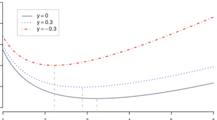
2.3 Expected execution cost uDH(T, x, Y) as a function of T for different values of trade imbalanceY. The dashed line indicate the value ofT achiev-ing the minimum. Figure drawn for β = .05, σ = .14, η = .05, κ = 10,

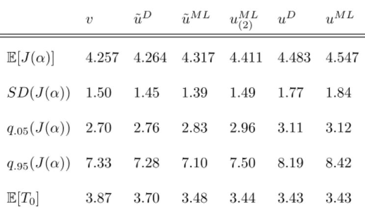
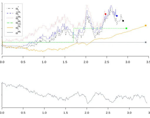
λ(x) = 0.1x2 and inventory x= 3. . . 46 2.4 Comparison of trading rates (αt) for each of six strategies in Table

3.1 given the shown simulated path of (Y0

t ) (The realized (Yt) depends on

the strategy chosen). Note that each strategy terminates at a different T0

indicated with a square. . . 50 2.5 Trading rates ˜αDL₍_{x, Y}_{) plotted as a function of flow imbalance} _y _for

different values of informational cost κ and information leakage strengthη. Inventory level is fixed at x= 3. . . 52 2.6 Left: Distribution of realized execution horizon T0 following strategy

˜

αDLfor different values of initial flow imbalanceY0. Statistics corresponding

to Y0 = 0 are given in Table 3.1. Right: Realized execution horizon T0

(13)

2.7 Top: 200 simulated trajectories (xt) from dynamic adaptive strategy

˜

αDL

t . Highlighted are three trajectories resulting from different realized

trade imbalance (Yt) paths. Bottom: Corresponding realizations of trade

imbalance t7→Yt. . . 55

2.8 The EWMA trade imbalance metric for Teva Pharmaceutical (ticker: TEVA) for a single day 5/3/2011. The data includes executed orders from Nasdaq, BATS and Direct Edge exchanges which accounted for 2,497,623 of the 8,059,668 total traded shares on the day. We also show the VPIN-like metric that used V = 25,000 and n= 20 in (2.33) and (2.34) respectively. 58 3.1 Stylized limit order book. . . 75 3.2 Best bid/ask queues v₁j(t) for TEVA along with bid/ask price pj₁(t) (top). Data taken from a 90 second window beginning at 2:30pm on 2/18/2011. Cancellations exceed additions at the best bid. Limit orders are in red and blue depending on side, market executions are orange. . . 79 3.3 Plot taken from Lehalle et al. [40]. Stock price P(t) for Coca-Cola and LOB volume imbalance V I(t) at the touch aggregated over 5 minute time bars (green/black). . . 81 3.4 Left: daily evolution ofP I_NA (upper) andP I_NB (lower) for MSFT,N = 80,000 over the first 50 trading days of 2011. Right: Histogram of P IA_,

measured at each execution time for a single day 1/4/11. . . 87 3.5 Left: Net order flow at the best bid level V LB_k. Right: Time elapsed during volume slices. Figures drawn for MSFT over 103 trading days. . . 88 3.6 Summary plots for TEVA for all 103 trading days. Left: Histogram of ∆Pk. Right: Price change ∆Pk plotted against trade imbalance T Ik

fitted-least squares regression line. . . 89 3.7 Left: ∆P against T I for TEVA over volume slices of V = 17,000. Right: Non-linear curves for MSFT, TEVA, BBBY were computed using penalized regression splines. The flatter curve in MSFT is due to its higher depth relative to the size of volume slice V. . . 91 3.8 Autocorrelation plots at minutes-scaleV = 1%ADV, 103 trading days. Left: V LA _and _{V L}B _{for BBBY. Right: Occurrence of scarce liquidity for}

TEVA. . . 103 3.9 Smoothed contemporaneous correlation betweenV LandV M over the past 2.5 hours using 30-second buckets with colors indicating different trad-ing days. Left: TEVA. Right: MSFT. Solid: bid-side. Dashed: ask-side . 104 3.10 T I plotted against net limit order flow at the bet bid (left) and best ask (right). Red (blue) points indicate volume slices with price decrease (increase) of at least .05. MSFT, covering the first 50 trading days of 2011. 105

(14)

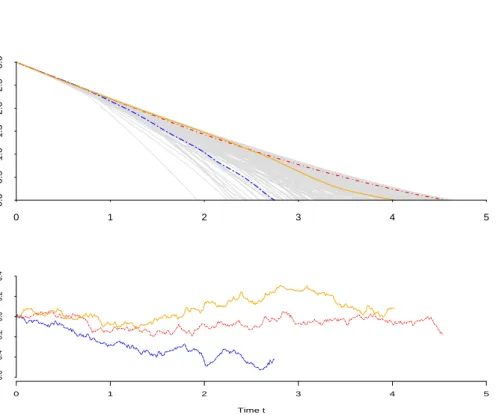
4.1 Optimal liquidation strategies (α`

t) (left) and (αct) (right) for 500

sim-ulated paths of expected trade imbalance (Yt). Baseline Almgren-Chriss

strategy is shown (bold solid line) along with colored bands corresponding to the 75%/25%, 90%/10% and 99%/1% quantile ranges. . . 123

(15)

Chapter 1 Introduction

1.1 Background

More than half of the markets in today’s financial world are electronic in nature and utilize some form oflimit order book (LOB) mechanism to facilitate trading. The speed, efficiency and transparency resulting from this market structure means that market participants are provided real-time access to the full LOB, and with it an extensive level of detail. This has contributed to the significant growth of automated or algorithmic trading, which now accounts for the majority of executed orders in many markets. Algorithms are developed via quantitative methods in order to satisfy the particular objective of some market participant. Possible objectives include the optimal liquidation of an asset while minimizing market impact, or providing liquidity

(16)

to the market (market making) while controlling for various risks. Once deployed, an algorithm incorporates a variety of real-time inputs from markets and executes orders automatically, without direct human involvement.

In practice, the development of strategies and algorithms relies heavily on the approach and corresponding assumptions in modeling market dynamics. The com-plexity of today’s market micro-structure has led to a wide variety of approaches with ideas from a number of disciplines including economics, statistics, mathematics and physics. Countless contributions have been made to the literature that focus on only a narrow slice of the overall LOB system. Such a limited scope is a necessary concession resulting from the high dimensionality of the LOB, complex interactions between many heterogeneous agents and interconnectedness of numerous exchanges and other trading venues, and other factors.

Work from the economics literature including early work Foucault et al. [29], Parlour et al. [47] and Easley et al. [25] tended to focus on the behavior of individual agents making rational choices, i.e. utility maximization, thus presenting the LOB as a type of sequential game. Not surprisingly, it is often difficult to recover many stylized features of actual markets when following this convention. An alternative approach from a math/physics perspective directly assigns stochastic dynamics to order flows or prices providing a convenient structure from which to analyze the features of the resulting system. The seminal work by Almgren and Chriss [5] for example originated

(17)

the framework of diffusive mid-price models, and others including Cont et al. [18], Alfonsi et al. [1] and Cartea et al. [17] have modeled price or order flow directly in lieu of building from the ground up with rational individuals. This second approach, which draws on a wealth of empirical studies into the statistical properties of price and order flow data, is often helpful in reducing the state-space complexity of the LOB and proves convenient for the purpose of designing algorithms.

Generally with a particular problem in view, one proposes a quantitative micro-structure model with features such as price, order arrival or LOB shape governed by stochastic processes, and then standard control techniques are utilized to solve for optimal strategies. There are two main classes of problems. The first is optimal liquidation, which is concerned with realizing the best value for the asset traded via optimization with respect to the incurred trading costs which are highly dependent on the method of execution. A traditional institutional investor with a large position in some asset would be acutely interested in the liquidity profile, average volume and price volatility of the asset over the course of multiple trading days. The second, is the problem facing a liquidity provider. Market making firms providing liquidity for a given asset are concerned with issues such as latency, and intricacies of order flow on a very short time scale on the order of a millisecond or less. The majority of quantitative academic work in algorithmic or high frequency trading are concerned with some variation of one of these two problems. A notable third objective is the

(18)

issue of market stability (see work by Kirilenko et al. [37] and Easley et al. [23]). The present work fits within the optimal liquidation context, but also explores in detail the assumptions and previous results from the literature related to the optimal behavior of liquidity providers.

1.2 The Limit Order Book

Prior to the introduction of LOB markets financial transactions took place in quote-driven environments in which a few designated market makers posted their bid and ask levels, respectively those prices at which they were willing to buy or sell. The market makers set the ask price higher than the bid price in exchange for supplying liquidity to the market and therefore assuming the risk of an unwanted long or short inventory position and the risk of adverse selection. Adverse selection has traditionally been described as a market maker’s encounter with an informed trader, one with better information about the fundamental value of the asset, but can also be described more generally as the instance when the price moves against the market maker following a trade. In a quote-driven market, traders are only able to trade immediately at the posted bid/ask levels. The LOB market structure on the other hand offers all market participants the ability to place buy and sell orders at any price.

(19)

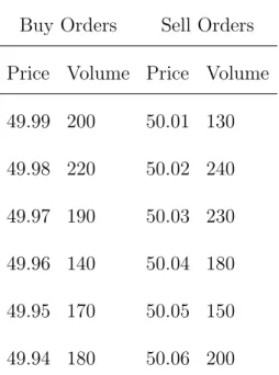
Buy Orders Sell Orders Price Volume Price Volume 49.99 200 50.01 130 49.98 220 50.02 240 49.97 190 50.03 230 49.96 140 50.04 180 49.95 170 50.05 150 49.94 180 50.06 200

Table 1.1: Hypothetical limit order book.

A limit order represents the interest to buy or sell a specific quantity of an asset at a specific price. The LOB is defined as the collection of all active limit orders and is discretized in terms of the tick size, typically 1 cent for US equities. The state of the LOB changes throughout the trading day as participants place new limit orders, cancel existing limit orders, or as market orders arrive and are matched to active limit order(s) through execution. Table 1.1 shows a snapshot of the synthetic LOB and Figure 1.1 shows the corresponding graphical representation.

While a limit order specifies the agent’s desired quantity and price, the timing of the execution is left uncertain if it occurs at all. On the other hand, a market order

(20)

V olume Price V olume Price

Figure 1.1: Left: Graphical depiction of the limit order book. Right: A market sell order (yellow) is matched against limit orders at the best bid levels.

represents the agent’s desire to buy or sell a certain quantity of the asset immediately. Upon arrival of a buy (respectively, sell) order for O shares, the trade-matching mechanism governing the LOB matches the order against the lowest (respectively, highest) priced active limit orders. Figure 2 illustrates one such interaction between a market sell order and the first O shares worth of active limit buy order(s).

For the right to guarantee immediate execution, the agent placing a market order, referred to as liquidity taker, receives slightly worse than the mid-price, at least one half of the bid-ask spread, depending on the volume of the order. The bid-ask spread is the difference between the highest priced limit buy order and the lowest priced limit sell order. Conversely, for supplying liquidity to the market, the agent placing the

(21)

limit order, the liquidity provider, receives slightly better than the mid-price, which in theory is compensation for taking on the associated adverse selection costs.

Beyond the idealized LOB framework presented above, various complicating nu-ances exist depending on the trading venue. Many exchanges allow participants to place fully or partially hidden orders, subject to certain rules varying by venue. This hidden liquidity is not visible to other participants but can be executed against arriv-ing market orders. Other examples include the method for establisharriv-ing priority for limit orders with the same price (eg price-time, pro-rata etc) and rebates, in which a small fixed fee is earned or paid for liquidity providers or takers respectively upon an execution. While each of these factors can have significant impact on trading strate-gies and the profit/loss of market participants, it is not uncommon to ignore many of these issues for the sake of mathematical tractability.

The LOB and related quantities will be defined more carefully in the empirical study in Chapter 3. For the moment it suffices to understand the general framework of the LOB mechanism and note that most problems on the topic are concerned with solving for optimal placement of limit and market orders given a specified model and objective.

(22)

1.3 Liquidity and Price Impact

The study of LOB dynamics is the study of trading frictions that are largely ig-nored by classical mathematical finance models. Though market dynamics clearly operate in discrete quantities, both in time (order arrivals, executions) and space (LOB, tick sizes), it is common to assume that trading, prices or liquidity dynam-ics are continuous. This approach often simplifies the mathematdynam-ics and allows for tractable strategies and solutions to be computed via stochastic calculus methods.

For a given asset, the amount of shares available for immediate purchase or sale at a given price, is limited. The result is that trading a large volume of the asset moves the price, usually in an unfavorable direction. The ease with which an asset can be bought or sold is referred to as the liquidity of the asset.

In the LOB context, an asset is said to have a high level of liquidity if a relatively large amount can be purchased or sold immediately (depth), the difference between the best bid and best ask prices is small (spread), and one can expect to buy or sell a large portion of the asset over time at a price not too much worse than the current price (resiliency) (Kyle, [39]). Yet, even for the most liquid of assets, transacting efficiently requires one to consider and model the asset’s liquidity dynamics.

There are several approaches in the math-finance literature to modeling liquidity from the perspective of the execution trader. For a large class of stocks, the bid-ask spread remains relatively constant (often at one tick) and is often assumed fixed in

(23)

order to simplify the model (See Dayri and Rosenbaum [20]). The depth and resilience of the LOB are typically captured through the model assumptions made related to price impact. Price impact links the volume of an executed order to the resulting change in price, and is often decomposed in the following categories:

Temporary Impact

Temporary or instantaneous price impact consists of the immediate effects of an executed market order. This impact is called temporary because it is assumed that the LOB will replenish quickly leaving the future price of the asset unchanged. Figure 1.1 highlights the consumption of limit buy orders that takes place upon arrival of a large market sell order. Clearly the average price received per share decreases as the order size increases, with the functional relationship dependent on the precise shape of the LOB. It is common for execution models [5] [4] [31] [16] to assume a continuous box shaped LOB (linear impact) which gives rise to the following transaction price

ˇ

Pt=Pt−καt,

wherePtis the fundamental price,αtis the order size andκis a nonnegative constant.

Note that impact in α affects only the current order, and does not affect Pt. The

total revenue of the trade is αtPˇt, yielding an execution “cost” of g(αt) = αt(Pt−

ˇ

Pt) =κα2t. This assumption is roughly consistent with empirical studies which have

(24)

[41]. Therefore, g must be convex to encourage the splitting of large orders into smaller pieces to be executed incrementally over time to reduce execution costs.

Permanent Impact

Permanent price impact on the other hand refers to the long term effects on the asset price. The size and frequency of market order arrivals conveys information that causes other traders to behave differently in the future. Of course, it is not possible to precisely measure the long-term impact of an action as it would require a comparison between a scenario that happened with one that did not. Studies focusing on the impact of individual trades or metaorders1 _{report concave (e.g. the so-called “square}

root law”) impact in the size of the order, see for example Lillo et al. [41], [45]. An alternate approach approximates permanent impact on an aggregate basis by relating trade imbalance, the difference between executed market buy and sell volume, with the corresponding price change over a set time interval. Price and trade imbalance often exhibit a linear relationship [13], [16]. Indeed, within the well known Almgren-Chriss framework, permanent impact must in fact be assumed linear for the model to be free ofprice manipulation2 [30]. For these reasons and for tractability it is common for optimal execution models to incorporate linear permanent price impact.

1_{A large order executed incrementally over time}

2_{Defined as a round trip trade, that is a series of trades with sum zero, with negative expected} costs.

(25)

Transient Impact

Transient impact refers to price impact that decays over time. In contrast to the above, transient impact evolves over time capturing elements of both temporary and permanent impacts. Implicit in the temporary framework discussed above, is that the LOB recovers instantly to its previous shape and subsequent transactions are not affected. Transient impact relaxes the instant recovery assumption by directly modeling the resilience of the limit order book. Linear transient impact was first considered by Obizhaelva and Wang [46] with several later extensions; Alfonsi et al. [3], Gatheral et al. [32] considered various decay kernels and Alfonsi et al. in [1] allowed for general LOB shape functions.

To sum up, most models that address the “optimal execution of a large investor” problem incorporate one or more of these price impacts. On the other side of the trade is the problem of how best to supply liquidity to the market. Several recent studies focus on the optimal order posting strategy for liquidity providers, including Cartea et al. [17] and Guilbaud and Pham [34]. In general, HFT market makers profit through the posting of buy and sell limit orders simultaneously and earning the spread whilst avoiding adverse price movements. A market maker strategy then might consider the depth (relative to the mid-price) or size of her limit order, the duration until cancellation (assuming execution does not occur immediately), and might adapt to the changing state of the LOB or the arriving market order activity. As market

(26)

maker strategy determines the shape and behavior of the LOB, understanding key factors that contribute to this strategy are crucial to properly model liquidity.

1.4 Information and Order Flows

It is well established in classic microstucture research [39], [25] that arriving order flows3 _{convey information to other market participants. Indeed, Bouchaud et al.}

[13] argue that endogenous changes in supply and demand, which are manifested in order flows, are more influential in the price formation process than exogenous information. Thus an understanding of how order flow is received and processed by markets and consequently asset prices is a requirement for efficient execution. The two base classes of trades are market orders and limit orders. Market orders indicate actual transactions taking place and hence ultimately drive traders’ P&L. Due to their intrinsic nature of “putting money on the table”, they carry the most information and are typically viewed as influential by other participants. Limit orders are posted by liquidity providers and serve as reference points in the price discovery process.

Several pathways have been proposed between order flow and liquidity/price move-ment. First, one-sided market order flow (MOF) is typically associated with a mov-ing market. Indeed, heavy market sellmov-ing will intrinsically tend to depress prices, mechanically by consuming the top queues of the LOB, and potentially by

(27)

ing new information about the fundamental value of the asset. As a result, extreme MOF would increase adverse selection and tends to reduce liquidity provision by mar-ket makers. Consequently, extreme MOF is expected to lead to scarce liquidity and increased price impact. Consider the following from Easley et al. [27]:

“...market makers adjust the range at which they are willing to pro-vide liquidity based on their estimates of the probability of being ad-versely selected by informed traders. Easley, Lopez de Prado and OHara [2012] show that, in high frequency markets, this probability can be ac-curately approximated as a function of the absolute [market] order im-balance...suppose that we are interested in selling a large [position] in a market that is imbalance towards sells. Because our order is leaning with previous orders, it reinforces market makers fears that they are being ad-versely selected, and that their current (long) inventory will be harder to liquidate without incurring a loss. As a result, market makers will further widen the range at which they are willing to provide liquidity, increasing our orders market impact...Thus, order imbalance and market maker behavior set the stage for understanding how orders fare in terms of execution costs.”

Market maker strategies must incorporate expected order flows (specifically MOF) and make adjustments in order to account for adverse selection costs or else risk lower profits. A similar result is obtained by Cartea et al. [17], who solve the optimal order placement problem for an HFT market maker. In response to rising adverse selection costs that coincide with increasingly one-sided MOF, the optimal strategy for the HFT market maker is to cancel any current orders and re-post deeper in the LOB.

Second, there are opinions that order flows summarize market sentiment and changing information set. Consequently, market news are encoded in order flow and the latter can be used to measure the influence of a given trade. For example, sudden

(28)

“news surprises” might manifest itself in rapid reversal of MOF, which in turn tends to depress liquidity as liquidity providers step back to reduce risk. This concept has been the motivation for defining toxicity indices, namely Easley et al. [23],[24], [26].

Third, order flow may indicate manipulative behavior of other participants. For example, the widely cited practice of “order fading” supposedly consists of rapid posting and cancellation of limit orders, to create a mirage of market activity and depth, in order to bait market orders and ultimately generate extra profits from round-trip profits. Similar strategies can be employed to front-run slower traders if the agent has speed advantages. The proliferation of latency arbitrage (see Kirilenko et al. [38]) suggests that these actions are quite profitable. In consequence, regular traders (and market regulators) are urged to monitor order flows to detect such patterns and manipulative actions.

To sum up, order flows can be used to estimate market trends (which would create asymmetric price impact), to detect increased market risk (that increases volatility or symmetric price impact), and to avoid manipulation (which implies that the LOB snapshot is not necessarily indicative of true market state due to latency arbitrage). All of this is crucially important to the execution trader who wishes to efficiently liquidate or acquire many shares via execution of a metaorder. Rather than simply assuming static liquidity or price impact function(s) described above, an execution algorithm ought to consider the typical behavior of HFT market makers and the state

(29)

of the liquidity provision process at the time of execution. How the trader’s executed metaorder compares to, and assimilates with the existing MOF process appears to be quite relevant to the liquidity and price impact trades will encounter.

1.5 Outline and Contributions

In Chapter 2, taken primarily from the recently submitted paper Optimal Exe-cution with Dynamic Order Flow Imbalance [11], the above concepts of information and order flows are bridged within a combined dynamic model. The basics of the Almgren-Chriss setup are maintained, including continuous trading and instanta-neous price impact that arises from market microstructure. However, also included is a novel stochastic factor (Yt) for (expected) market order flow, which is similarly

im-pacted from executed trades. The transient impact onY represents the informational footprint of the trader and introduces a feedback loop into the problem. It allows the trader to react to changing market conditions, in particular markets changing from being buy-driven to ask-driven and vice versa. The model is used to examine the dynamic problem of Optimal Execution Horizon that was introduced in a 1-period version by Easley et al. [27]. Thus, in contrast to Almgren-Chriss and typical exe-cution models, the exeexe-cution horizon is endogenized, optimally chosen depending on market liquidity.

(30)

Intuitively, trading should slow down when informational costs are high, and speed up when they are low. From that point of view, rather than a pure optimization problem, optimal execution is about trading-off price impact and information leakage against timing risk. Moreover, endogenizing execution horizon generates dynamic execution strategies even if the underlying asset value is a martingale. This allows for inherently adaptive trading in contrast to early models with deterministic strate-gies (e.g. [2, 5, 8]) that consider only price impact. Some more recent extensions by Gatheral and Schied [31] and Almgren and Lorenz [6, 43] do produce dynamic strate-gies which are “aggressive-in-the-money”, accelerating when the price is rising. The approach in Chapter 2 on the other hand adapts to the changing state of liquidity and informational costs.

Chapter 3 then investigates several of the assumptions related to liquidity and execution costs made in [27] and Chapter 2 through an empirical study on Nasdaq data. Much of the recent literature on LOB dynamics operates in the extremely short timescale (1 second), analyzing the predictive power available by conditioning on the state of the LOB (e.g. Huang et al. [35], Donnelly [21], Cont et al. [18] and Lipton et al. [42]. Indeed, part of what makes the analysis of LOBs so challenging are the multiple timescales that apply, ranging from millisecond dynamics up to inter-day trends which span days or weeks. The analysis in Chapter 3 focuses on the minutes timescale at which optimal execution scheduling takes place. At this level, rather

(31)

than the state of the LOB, order flows are the main driver in price formation. This chapter aims, through statistical analysis, to understand the link between order flows and liquidity, with a particular focus on periods of scarce liquidity.

Finally, Chapter 4 revisits the optimal execution problem with several of the em-pirical results from Chapter 3 in mind. When the asset is a liquid stock, the model in Chapter 2 can be refined so that the informational costs related to expected trade imbalance (Yt) can be made more precise. Where costs are initially left general

and not directly mapped to the profit/loss of the trader, in Chapter 4 we explic-itly include the asset price and solve the optimal control problem with the trader’s wealth process as the objective function. Expected order flow enters the model in two places: (1) Through an additional cost when competing for scarce liquidity, and (2) In price dynamics, capturing the effect on the mid-price of limit order flow and LOB resilience/fading.

Ultimately we find that limit order flow is a key element in the price formation process. In contrast to the picture of a stationary LOB that replenishes following each execution, we instead observe periods of strong resilience (limit additions) and other periods characterized by little to no resistance in the LOB (rapid cancellations). It is shown that limit order flow is strongly linked with the arriving market order flow. Therefore, incorporating the expected trade imbalance Yt offers key insights into the

(32)

Chapter 2 Optimal Execution with Expected

Trade Imbalance

The concept of optimal execution in financial markets is concerned with realiz-ing the best value for the asset traded via optimization with respect to the incurred trading costs. These costs are driven by two fundamental components: market mi-crostructure frictions and informational asymmetries. Market mimi-crostructure implies that market liquidity is finite and trades generate price impact. Informational costs reflect the fact that trades are observed by other participants who will then adjust their own strategies and views of the asset value and create adverse selection.

Specifically, trading in a LOB leaves a double footprint, both in space and in time. In space, an executed sell order consumes the matching standing limit orders on the

(33)

bid side. (In our framework since there is no fill risk all trades are assumed to be market orders.) This shortens the respective queues on the bid side of the book and hence can move the best-bid. This is the previously mentioned temporary price impact represented by g(·). Temporally, the executed order is recorded by other participants on the exchange message ticker affecting the observed order flow. The effect is both direct (the immediate fact that a sell order of αt shares was executed), and indirect

(the fact that market participants adjust their statistical view of the order flow over time). Thus, to the extent that market participants monitor the ticker (rather than just observe the snapshots of the LOB), an order generates informational footprint. There is a lot of anectodal evidence that many HFT algorithms indeed track the time series of orders placed (for example to detect temporal trading patterns) and hence will react to this footprint. This implies that information costs are at least as important as instantaneous liquidity consumption.

Modelling order flow remains in its early stages. Indeed, while spatially the LOB can be easily summarized as a collection of queues (modeled via say the depth function [2]), the time series of the exchange ticker are much more complicated as market participants process multiple streams of information. There are both executed trades (i.e. trades triggered from market orders) and limit orders, which themselves can be added, cancelled, or modified in other ways depending on the exchange. Orders further carry volume, time stamp and possibly participant type (and limit orders can

(34)

be entered at any level of the LOB). These multi-dimensional data is moreover coupled in nontrivial ways, with temporal links both within series (e.g. auto-correlation in the inter-order durations) and across series (e.g. executed market orders tend to increase the arrival rate of limit orders at the touch). See for example a recent model of Cartea et al. [17] who fitted cross-exciting Hawkes processes to the basic order flow at the best-bid and best-ask queues. See also [36] and Cartea and Jaimungal [16] which we revisit in Chapter 4.

In the optimal liquidation literature, very few models consider costs related to tem-poral order flows and the resulting informational costs. A notable exception is the paper by Easley et al. [27], in which the optimal execution horizon is obtained by min-imizing information leakage (the amount by which the trader perturbs the expected market order flow process) subject to timing cost (see Section 2.3.3 for further discus-sion). The current chapter aims to extend this model [27] to a dynamic, continuous-time framework comparable to popular approaches such as Almgren-Chriss, while capturing both microstructure frictions and informational costs.

2.1 The Optimal Execution Problem

The problem in view is liquidation of a position of size x0 = x. We assume a

continuous-time setup, with trading taking place continuously and via infinitesimal amounts. Namely, the trader trades ˙xtdt shares at time t, so that his inventory xt

(35)

follows the dynamics

dxt= ˙xtdt. (2.1)

Execution ends at the random horizon

T0 := inf{t ≥0 :xt = 0},

whereupon inventory is exhausted. Throughout, time is supposed to be in traded-volume units.

Beyond the inventoryxt, the main state variable of our model is the expected trade

imbalance Yt. The trade imbalance captures the intrinsic fluctuations among supply

and demand for the security realized by the unequal amounts of buyer- and seller-initiated trades. On the short time-scale (intra-day to several days) it is empirically quasi-stationary, in the sense that the observed volume is several orders of magnitude larger than the deviations in net imbalance, cf. Section 2.4.1. Moreover it is highly noisy and appears to be mean-reverting to zero. Therefore, we choose to model (Yt)

in terms of a mean-zero stationary process.

Let Y0 _{represent the flow imbalance in the absence of the trader. As a}

start-ing point we take (Y0

t ) to be an Ornstein-Uhlenbeck process with mean-reversion

parameter β,

(36)

The mean-reversion strength β controls the time-scale of the memory in flow imbal-ance, while the volatility σ controls the size of fluctuations in flow imbalance. Since imbalance is intuitively in the range [−1,1] (representing markets with 100% buyers, and 100% sellers respectively), the fraction σ2_/₍₂_β_{), which is the stationary variance}

of Y0, should be on the order of σ2/(2β)∈[0.01,0.2].

The execution program of the trader introduces a downward pressure on the ex-pected trade imbalance process as a result of his selling. The information leaked by the trader’s action creates a drift in the realized order imbalance Yt, pushing it

below Y0

t . By displacing other orders, the trader impacts expectations regarding

fu-ture order flows and generates adverse selection. A more precise description of this mechanism using (more realistic) discrete-time setup and discrete trades is presented in Section 2.4.3. We postulate that

dYt =−βYtdt+φ( ˙xt)dt+σdWt, (2.3)

where φ(·) captures the information leakage. Observe that

Yt=Yt0+

Z t 0

eβ(s−t)φ( ˙xs)ds, (2.4)

so the execution program generates an exponentially decaying impact on Y0. We assume that φ:_R+→R+ is non-decreasing withφ(0) = 0. The three main cases we

consider are: φ( ˙xt)≡0 corresponding to zero informational footprint; φ( ˙xt) =φt

(37)

φ( ˙xt) = ηx˙t. Linear impact is computationally convenient, though not necessarily

the most realistic reflection of how a trader’s activity might influence expectations regarding order flow. Impact that depends on the current value of the flow imbalance is investigated in Section 2.4.3.

Remark 1. Below we restrict our attention to pure selling strategies, so thatxtis

non-increasing. As such all our cost functionals are only defined for positive selling rates. Depending on the strength of information leakage, it is possible that the constraint

−x˙t ≥ 0 is binding, i.e. execution is suspended until market conditions improve.

It is beyond the scope of this paper to extend the framework to two-sided trading algorithms that raise the issue of potential market manipulation [3, 32].

The information leakage is “abstract” in the sense that it does not generate trading costs per se. However, in line with [27] we assume that there are adverse selection costs associated with trading in an unbalanced market. Here we assume that this cost is symmetric inYt (but note that agent’s actions induce only one-sided effects of

Yt); for tractability we take it quadratic. Whether the sign ofYt should more heavily

influence costs is a valid question that we revisit in Chapter 4.

In addition, we carry through two usual costs from the literature. The Almgren-Chriss model [5], detailed in Lemma 2.2.1 below, serves as a baseline strategy in our analysis. This classical model is characterized by two execution costs which we also adopt: instantaneous impact g( ˙xt) of trading at rate ˙xt, and inventory costλ(xt) for

(38)

carrying a position of xt at t. In this chapter we make the assumption (as in [5])

that the asset price is a martingale and therefore does not enter the proceedings. Permanent market impact is modelled via the informational effect on Yt rather than

on the asset price directly.

The continuous-time execution problem is to minimize the sum of the correspond-ing expected execution costs

inf (xt)∈X(x)E x,Y Z T0 0 g( ˙xs) +κYs2+λ(xs) ds , (2.5)

over admissible execution strategies (xt) ∈ X(x). The above expectation is

condi-tional on an initial value Y0 = Y and initial inventory x which induce the measure

Px,Y. The horizonT0 is part of the solution, so that the optimization is formally

tak-ing place on the whole futures∈[0,∞). We assume for the duration thatg( ˙x) = ˙x2_.

This first term in (2.5) incentivizes the trader to slow down in order to reduce his immediate liquidity costs while the next two terms of the cost functional are such that under certain market conditions, it may be optimal to accelerate trading in order to exit the market sooner.

LetFt=σ(Ys:s≤t) denote the filtration generated byY. Admissible strategies

(xt) ∈ X(x) consist of (Ft)-progressively measurable, absolutely continuous

trajec-tories t 7→ xt, such that x0 = x, limt→∞xt = 0 and

R∞

0 x˙

2

sds < ∞ P-a.s. We also

require the following assumptions on the model ingredients:

(39)

• The informational cost parameter κ≥0;

• Inventory risk λ:_R+7→R+ is non-decreasing in x.

The cost functional in (2.5) is consistent with other approaches taken in the lit-erature. The assumption that g( ˙x) is convex matches the empirical fact that market participants like to divide a large “parent” order into smaller orders in order to re-duce trading costs. In LOBs, g(·) represents the depth of the LOB on the ask-side. If this depth is constant, the instantaneous trading cost is quadratic g( ˙x) = ˙x2 _(by

rescaling κ and λ we assume without loss of generality that the leading coefficient is 1). This assumption also appears in [5, 15, 31] among others. Because our primary focus is on informational costs, we assume for the moment that there are no other transient/permanent impacts on the asset value Pt and further posit that strategies

are independent of asset dynamics. In Section 2.4.2 we return to this issue and discuss extensions that allow for positive correlation between asset price dynamics (Pt) and

order flow (Yt).

Our second cost term κY2

t is motivated primarily by the model presented in [27]

and captures the cost of information leakage. The main premise is that liquidity costs (e.g. likelihood of adverse selection) are higher in markets with unbalanced flow. Unlike [27], our model incorporates stochasticity and mean reversion in the flow imbalance process (Yt), meaning that the impact modelled with this term is transient.

(40)

Other models incorporating transient impact have focused on LOB resilience [2, 32]. Also see [4] for another example of stochastic liquidity costs.

The last termλ(xt) in (2.5) represents timing risk, penalizing the trader for leaving

his position exposed to adverse price movements. Several risk terms have been applied within the execution literature. The seminal work by Almgren and Chriss, which optimizes over a mean-variance cost functional, reduces to a calculus of variations problem and the risk termλ(x) = cx2. Gatheral and Schied [31] investigated a time-weighted value-at-risk measure proportional to λ(x) = cx. In the context of timing risk, λ(x) = c generates costs that are proportional to execution time which is a non-trivial modification once the horizon T0 is not fixed.

Remark 2. Other authors refer to order imbalance for a different object, namely “spa-tial” order imbalance. Namely, motivated by queueing notation, they mean the net difference between standing limit orders at the best-bid and best-ask. As shown by [42] and [21], order imbalance is predictive of the next price move (i.e. correlated with the probability of the next price to be an up-tick or a down-tick) and is closely mon-itored by most HFT algorithms. In this chapter we focus on the temporal order flow and its associated imbalance that was conjectured by Easley et al. [23, 24, 27] to be related to market toxicity. While the LOB depth is related to the history of submitted limit orders, the relationship is highly complicated (due to shifting mid-price, hidden orders, etc.). Consequently, our trade imbalance is not meant to be tied directly to

(41)

the LOB depth or any immediate LOB properties, but rather provide a temporal sum-mary of recent orders submitted. Further, we make the important distinction that process (Yt) is the expected trade imbalance, that is, the trade imbalance that

mar-ket participants are expecting. This quantity is closely related to the observed trade imbalance that summarizes recent order flows, but the exact relationship between the two is difficult to pinpoint. Section 2.4.1 discuss further.

2.1.1 HJB Formulation

To minimize (2.5) we adopt the standard stochastic control approach, utilizing the dynamic programming principle and Hamilton-Jacobi-Bellman (HJB) PDE. Within this framework strategies are defined by their rate of selling, αt:=−x˙t and the class

of admissible strategiesA(x) consists of all nonnegative (Ft)-progressively measurable

processes (αt)0≤t≤T0 for which

xα_t := x− Z t 0 αsds + , 0≤t,

belongs toX(x). The value function of our problem can be expressed as

v(x, Y) = inf (αt)∈A(x) Ex,Y Z T0 0 g(αs) +κYs2+λ(xαs) ds . (2.6)

If it exists, we define the corresponding optimal strategy asα∗(x, Y). For each path of underlying Y0

t ,α

∗ _{induces the realized execution horizon}_T

0(x, Y) = inf{t :xα ∗

t = 0}

(42)

One key point of interest is the realized execution horizon that results from the optimal dynamic strategy, which can only be obtained by solving (2.6). To this end, we assume that v is sufficiently smooth, and apply the dynamic programming principle which says that

t7→v(xα_t, Yt) +

Z t 0

α2_s+κY_s2+λ(xα_s) ds

ought to be a submartingale for all α and a martingale when α is optimal. Then, an application of Itˆo’s formula suggests that the value function v(x, Y) will satisfy a Hamilton-Jacobi-Bellman equation of the form

0 = 1 2σ

2

vY Y −βY vY +κY2+λ(x) + inf

α≥0{g(α)−αvx−φ(α)vY}, (2.7)

with the boundary conditionv(0, Y) = 0 for allY. We observe that (2.7) is a nonlinear parabolic PDE in (x, Y) for which the corresponding theory (e.g. regarding existence of classical solutions) is rather limited.

When instantaneous price impact cost is quadratic g(α) = α2 _{(assumed for the}

remainder) and information leakage is linear φ(α) =ηα, the candidate optimizer in feedback form is

α∗(x, Y) = vx+ηvY

2 . (2.8)

Substituting this feedback control into the PDE (2.7) we have 0 = 1 2σ 2 vY Y −βY vY +κY2+λ(x)− vx+ηvY 2 2 . (2.9)

(43)

Due to the state dependence of the class of admissible strategiesA(x), the problem (2.6) is a finite-fuel control problem. As a result, there does not appear to be a tractable closed form solution which satisfies the zero boundary condition along x= 0. In Section 2.5 we illustrate a relatively straightforward method for solving (2.9) numerically via a finite difference scheme.

To understand the feedback strategy in (2.8), we pause to consider the derivatives

vx and vY. As we will see, vx is always positive but vY can be either positive or

negative. Consequently, the candidate in (2.8) may fail to be non-negative. Lemma 2.1.1. The map x7→v(x, Y) is strictly increasing for any Y.

Proof. Fixx < x0 =x+for a strictly positiveand consider an (-optimal) strategy

α _for _v₍_x0_{, Y}_{). Let} _T

x := inf{t:x0t =}be the random period to sell x shares using

α_{. Then by absolute continuity of} _t _7→ _x0

t, Tx < T0(x0, Y). Moreover, α0(x, Y) :=

α_t(x0, Y)1{t≤Tx} is an admissible strategy for the initial conditions (x, Y) since it

liquidates exactly x0−=x shares. Using the fact that α0 is sub-optimal forv(x, Y) and that the second and third terms in (2.5) are strictly positive almost surely, we find v(x, Y)≤v(x0, Y;α0)< v(x0, Y).

In (2.9), the horizon is indefinite and ultimate liquidation is only modelled through the boundary condition. Thus, understanding the realized execution horizonT0(x, Y)

is only possible implicitly. Moreover, the nonlinearities in (2.9) make analysis in-tractable. To achieve tractability we consider an approximate two-stage procedure.

(44)

Thus, we first fix a horizon T by imposing the constraint T0 = T. We then solve

the resulting fixed-horizon problem to find the best strategy α∗(T, x, Y) and value function v(T, x, Y). In the second step, we optimize over T, to find the statically optimal horizon T∗(x, Y). Finally, we build the semi-dynamic strategy ˜α(xt, Yt) =

α∗(T∗(xt, Yt), xt, Yt). Thus, ˜αrecomputes T∗ as the state variables (xt, Yt) evolve and

uses the corresponding static trading rate. This approach is analogous to the receding-horizon setup in nonlinear control [48]. Indeed, the initial use of α∗(T∗(x, Y), x, Y) att= 0 corresponds to model predictive control and ˜α(xt, Yt) then continuously rolls

the initial condition because of the stochastic fluctuations encountered. The above plan is implemented in Sections 2.2 and 2.3 respectively. In the latter section we also compare the execution trajectories and resulting costs from the various strategies.

2.2 Linear Quadratic Setup on Finite Horizon

Fix T < ∞. We consider the analogue of (2.6) on [0, T]. To avoid confusion we letu denote the value function when defined on the fixed horizon:

u(T, x, Y) = inf (αt)∈A(T ,x) Ex,Y Z T 0 α2_s+κY_s2+λ(xα_s)ds . (2.10)

For expository purposes, we use the time-to-maturity parametrization for u so that the first argumentT represents timeuntil the deadline. Strategies on [0, T] are defined in similar fashion to those in Section 2.1 but with a constraintxT = 0 at the terminal

(45)

time T. Forced liquidation by T is achieved by leveling an infinite penalty if not completed, leading to a singular initial condition of the form

lim T↓0u(T, x, Y) =          0 if x= 0 +∞ if x6= 0. (2.11)

To obtain explicit solutions to (2.10), the next section treats the case in which

φ is independent of α over a fixed horizon. In other words, the trader may or may not impact the order flow process, but any impact can be modelled in a deterministic fashion. Section 2.2.2 then addresses the proportional footprint φ(α) =ηα case, still over fixed time horizon. It will be shown that the strategies obtained in Sections 2.2.1-2.2.2 are not too suboptimal compared to the indefinite-horizon model laid out in Section 2.1.

2.2.1 Myopic Execution Strategies

In classical optimal execution models [2], [5] and [8], optimal execution rates are deterministic, i.e. αt is pre-determined. In this scenario, informational costs would

also be deterministic. Therefore, we examine the case where φ(α) is independent of

α (but possibly depends on time t). So (Yt) takes on the dynamics

(46)

Under this assumption, we can separate the two terms in (2.5) since the dynamics of (Yt) are not directly affected by the trader; the performance criterion simplifies to

inf (xt)∈X(x) Z T 0 ˙ x2_s+λ(xs)ds + Z T 0 κ_EY[Ys2]1{xs>0}ds. (2.12)

Because (Yt) is independent of the controlα, optimal strategies are defined only by the

first term in (2.12). Consequently, the resulting (αt) is independent of Yt and hence

t 7→ x∗_t is deterministic. Thus, strategies based on (2.12) are myopic in the sense that they entirely ignore the potential “footprint” left by the trader’s actions, instead focusing solely on instantaneous cost and inventory risks. The following Lemma provides the solution to (2.12) for popular choices of inventory risk.

Lemma 2.2.1. Consider the calculus-of-variations problem of finding

I(T, x) := inf

(xt)

Z T 0

( ˙x2_t +λ(xt))dt

where the minimization is over all absolutely continuous curves t 7→xt with x0 = x,

(47)

strategies (with αt≡ −x˙t) are                  xM L_t = x(T −t) T ; α_tM L= x T; IM L₍_{T, x}_{) =} x 2 T ,                  if λ(x) = 0; (2.13)                    xM H_t = xsinh( √ c(T −t)) sinh(√cT) ; αM H_t = √ cxcosh(√c(T −t)) sinh(√cT) ; IM H₍_{T, x}_{) =}√_cx2_coth(√_cT₎_,                    if λ(x) = cx2; (2.14)                                  xM Q_t = ct 2 4 −t cTˆ 4 + x ˆ T ! +x ! 1{t<Tˆ}; αM Q_t = cTˆ 4 + x ˆ T − ct 2 ! 1{t<Tˆ}; IM Q₍_{T, x}_{) =} ₋c2Tˆ3 48 + cT xˆ 2 + x2 ˆ T ! ; where Tˆ:= min(T,2 √ x √ c ),                                  if λ(x) =cx. (2.15)

Proof. See Section 2.5

The superscriptsM L, M Q, M Hrespectively stand for the Myopic Linear, Quadratic and Hyperbolic models. The first case ML yields linear selling and the TWAP strat-egy, or if time is parametrized in volume time, the classic VWAP trading strategy. The second strategyxM H

t and its corresponding rateαtM H represents exponential

(48)

This risk term results from the trader’s effort to minimize the variance of liquidation cost. From the perspective of an inventory risk measure, one natural alternative is

λ(xs) =cxs, which has the attractive property of being proportional to value-at-risk

and results in a selling strategy xM Q_t that is quadratic in t. Yet as explained for a similar problem in [31], buying might result with position size small relative to T. Imposing the constraint that xM Q_t is decreasing then leads to the modified solution (2.15) which in the case ˆT < T causes liquidation to end prior to the terminal time

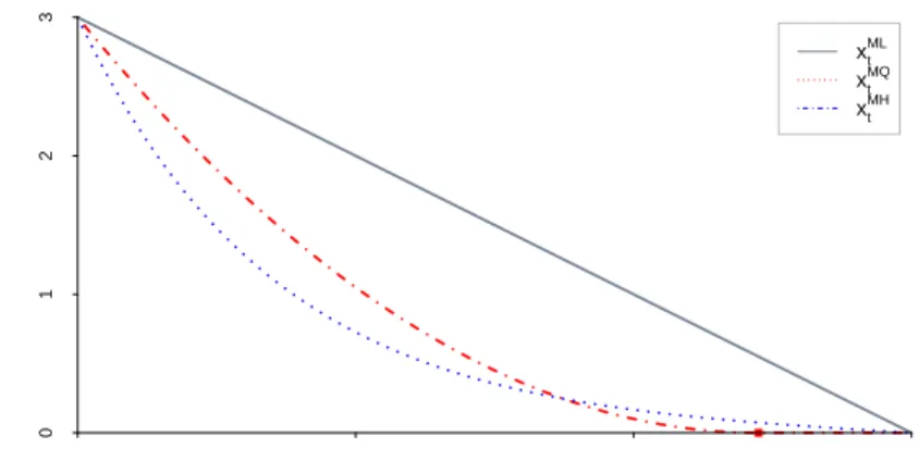
T. Time t In v e n to ry xt 0 1 2 3 0 1 2 3 x_tML x_tMQ x_tMH

Figure 2.1: Optimal trajectories from Lemma 2.2.1. Figure drawn for initial inventoryx= 3, horizonT = 3, andc= 2. This leads to ˆT =2

√

x

√

c = 2.45 in the quadratic scenario x

M Q _{of (2.15).}

Figure 2.1 details the three execution curves described in Lemma 2.2.1 for x= 3 andT = 3. Compared to the VWAP strategyxM L_{, the non-zero inventory risk terms}

(49)

rate in xM H _{is proportional to} _x_{, cf. (2.14) and liquidation occurs exactly at} _T_{. In}

contrast, as xM Q_t becomes small, the linear risk term cxM Q_t becomes more punitive and it may be optimal to end liquidation prior to timeT. Figure 2.1 shows inventory

xM Q_t reaching 0 at time ˆT =√6 as defined in (2.15).

We now turn our attention to the expected execution costs which arise from the trade imbalance. Fixing (α∗_t), we can view the corresponding information impact

φ(α_t∗) also as a deterministic function of t, allowing direct evaluation of the second term in (2.12) using the explicitly available Gaussian distribution of Yt.

Lemma 2.2.2. Given a deterministic, time-dependent flow impact φ(αt) = φt, and

Y0 =y, Yt has the second moment Ey Y_t2=µ2_t +σ_t2, (2.16) where          µt=ye−βt− Z t 0 e−β(t−s)φsds, σ_t2 = σ 2 2β(1−e −2βt₎_. (2.17)

Proof. To solve the SDE (2.3), we start with

f(Yt, t) =Yteβt

which after applying Itˆo’s formula gives

df(Yt, t) =βYteβt+σeβtdYt

(50)

Then integrating each side from 0 to t and dividing through by Yt on each side we have Yt =ye−βt+ Z t 0 eβsφsds+e−βt Z t 0 σeβsdWs

SoYt is clearly Gaussian with mean and variance as given in (2.17).

Putting everything together we obtain the expected total cost for the family of myopic execution strategies in Proposition 2.2.3. We reiterate that while realized costs instantaneously depend on the stochastic process (Yt), strategies in this section

are purely deterministic and do not adapt to (Yt). The solutions below are labeled

according to the form ofλ(x); while formally the two terms in (2.12) are decoupled, it is of course logical to match the resulting solutionI of the instantaneous price-impact part with the corresponding expectation of_Ey[

RT0

0 Y

2

s ds], which is the convention we

follow in Proposition 2.2.3.

Proposition 2.2.3. Suppose that φt(α) = φt. The corresponding value functionu is

given by

(51)

where I is defined in (2.13)-(2.15) and O = κ Z Tˆ 0 (µ2_t +σ2_t)dt (with Tˆ, µt and σt2 from Lemma 2.2.2) is O0₍_{T, x, Y}_{) =} κy 2 2β 1−e −2βT +κσ 2 4β2 2βT +e −2βT ₋₁ if φt ≡0; (2.19) OM L₍_{T, x, Y}_{) =}_O0₍_{T, x, Y}_{) +} κηxy β2_T 2e −βT ₋₁₋_e−2βT (2.20) + κη 2_x2 2β3_T2 2βT + 4e −βT ₋_e−2βT ₋₃ if φt =ηαM Lt

Closed form expressions are also available for OM Q _and _OM H_{, see Section 2.5.}

Thus, the overall cost of liquidation has two components: the I(T, x) term that depends only on (T, x), and the informational footprint term O(T0, x, Y) that also

depends on y. Recall that informational costs accrue only up toT0; in the linear and

hyperbolic cases we always haveT0 ≡T, but in the quadratic case liquidation may be

completed early, T0 = ˆT < T, see Figure 2.1. In terms of x, O is constant if φt = 0,

linear if φt = ηαM L, and quadratic otherwise. As a function of y, O is quadratic

thanks to the linear dynamics of (Yt) and quadratic informational cost. Financially,

they2 _{term represents higher costs due to trading in an unbalanced market, while the}

y-term adjusts to the fact that selling in a market dominated by buyers is favorable to competing with other sellers for scarce liquidity. The following Corollary shows that the “best” level of y is positive (or 0 if φt = 0). Intuitively, it is best to begin

trading in an environment with positive order flow so that the trader’s selling activity pushes the order imbalance towards 0 and reduces informational costs.

(52)

Corollary 2.2.4. Suppose that φt(α) =φt≥ 0. Then the flow imbalance that

mini-mizes expected execution cost is non-negative, arg minY {u(T, x, Y)} ≥0for anyT, x.

Proof. As already discussed,uM₍_{T, x, Y}_{) is quadratic in}_y _{and the coefficient of}_y2 _is

κ

2β 1−e

−2βT

. By inspection it is positive. The dependence on y comes from theO

terms that are of the form

O(T, x, Y) =κ

Z T 0

(Y e−βt−At)2 +σt2dt

where At ≥0 (strictly positive as soon as φt >0 on an interval of positive measure,

cf. (2.42)). It follows that the coefficient ofY2 inuM(T, x, Y) is κR₀T e−2βtdt >0 and of Y is −RT

0 2κe

−βt_A

tdt ≤ 0. Thus, setting ∂YuM(T, x, Y) = 0 and solving for Y

yields a non-negative result.

2.2.2 Dynamic Execution Strategies

We now return to the problem in (2.10), lettingφ(αt) =ηαt. The optimal dynamic

strategy is adapted to the expected trade imbalance process (Yt) and the trader’s rate

of selling directly influences (Yt). To avoid confusion we will denote dynamic strategies

and expected costs by αD

t and uD, respectively. The HJB PDE for uD(T, x, Y) is

uD_T = 1 2σ

2_uD

Y Y −βY uDY +κY2+λ(x) + inf α≥0

g(α)−αuD_x −ηαuD_Y , (2.21) with uD₍₀_{, x, Y}_{) = +}_∞ _unless _x _{= 0. Note that (2.21) is identical to (2.6) but for}

(53)

to the time-dependence arising from the constrained horizon T. Additionally, with the fixed horizon T, there is no boundary condition in x, meaning it is possible that trading could continue beyond the point at which inventory first reaches 0. Assuming

g(α) = α2_{, λ}₍_x_{) =} _cx2_{, and inserting the feedback control as in (2.9) yields a}

semi-linear, parabolic PDE

uD_T = 1 2σ 2_uD Y Y −βY u D Y +κY 2₊_cx2 ₋ uD x +ηuDY 2 2 . (2.22)

with initial condition (2.11). To obtain (2.22), it is necessary to letαbe unconstrained and allowed to become negative. This allows us to find the following candidate solution by exploiting the linear-quadratic structure. The motivation comes fromuM

in Proposition 2.2.3 where we find a similar result: quadratic in xand Y with an xY

term that adds additional costs when Y <0.

Proposition 2.2.5. The solution of (2.22) has the form

(54)

where D(T) = E(T) ≡ 0, A, B, C, F solve the matrix Riccati ordinary differential equations (ODEs)                              A0(T) =−A2₋_ηAC₋ η2 4 C 2₊_c B0(T) =−η2_B2₋_B₍_ηC _{+ 2}_β_{) +}_κ₋ 1 4C 2 C0(T) =−η₂C2₋_C₍_η2_B₊_A₊_β₎₋₂_ηAB F0(T) =σ2_B, (2.24)

and we have the following initial conditions

         lim T↓0A(T) = +∞ B(0) = C(0) =F(0) = 0. (2.25)

The optimal rate of liquidation is

αDH_t (T −t, xt, Yt) =

xt(2A(T −t) +ηC(T −t)) +Yt(C(T −t) + 2ηB(T −t))

2 .

(2.26)

Proof. See Section 2.5.

We reiterate that in (2.4.2) A, B, C, F are functions of time remaining and that we have simplified the notation by omitting the time argument (i.e.A0 =A0(T), etc.) on the right side of (2.4.2). Close to the deadline T, the impact from impacting Y

(55)

observed by formally linearizing the Riccati system (2.4.2) in the regime T −t =

and using the initial conditions (4.11). We obtain the following expansions in :

                             A() = 1 +O() B() =κ+O(2_); C() =−ηκ+O(2_); F() = σ2₂κ2 +O(3₎_. (2.27)

Inserting into (2.26) gives the short term trading rateαDH(, xt, Yt) = xt+O(). This

heuristically confirms that the strategy (2.26) is admissible which can also be observed in Figure 2.4 below: as t → T, the dynamic trading rate stabilizes, resembling a VWAP strategy.

Remark 3. It is also possible to set up and solve linear quadratic problems for other functional forms of inventory risk λ(x). In the constant case λ(x) = c the Riccati system is almost the same as (2.4.2) (again E(T) = D(T) ≡ 0) except that the c

term moves to the fourth line: F_DL0 (T) = σ2B(T) +c. In the linear case λ(x) = cx, the resulting Riccati system is

(56)

                                                 A0(T) =−A2₋_ηAC₋ η2 4 C 2 B0(T) =−η2_B2₋_B₍_ηC_{+ 2}_β_{) +}_κ₋1 4C 2 C0(T) =−η 2C 2₋_C₍_η2_B ₊_A₊_β₎₋₂_ηAB D0(T) =c−A(D+ηE)− ηC 2 (ηE +D) E0(T) =−βE−ηB(D+ηE)− ηC 2 (ηE+D) F0(T) =σ2_B₋ 1 4(ηE+D) 2_,

with initial conditions as in (4.11) and D(0) = E(0) = 0. However, dynamically satisfying the constraintx≥0 is not tractable (cf. ˆT in (2.13)) and we found that the resulting unconstrained strategies tend to lead to wild buying-and-selling. Notably, inventory xt often becomes negative in which case the inventory risk term loses its

meaning.

The equations in (2.4.2) can be dealt with using a software package such asR. It is however necessary to replace the singular initial condition (2.11) with the condition

lim T↓0u D (T, Y, x) =          0 if x= 0 M if x6= 0 (2.28)

for a constant M large, essentially allowing for a non-zero position at time T which must then be liquidated in a single order at some additional cost. This is equivalent

(57)

to introducing a boundary layer [0, ] and solving onT ∈[,∞] whereupon M = 1/

is the right choice based on (2.27).

The optimal trading rate αD _{in (2.26) is linear in both} _x

t and Yt. The former

feature is similar to the hyperbolic situation in (2.14) whereαM H

t is also linear in xt.

We next illustrate how the dynamic strategy αD_t compares to its myopic counterpart

αM

t . With fixed terminal timeT, the incentive for the trader to speed up or slow down

under strategyα_tD arises from the trader’s desire for more balanced order flow. Note that there is no incentive to accelerate one’s trading in order to exit the market prior to time T since costs from Y accrue until T. For positive trade imbalance, trading more quickly in the present results in lower execution costs in the future because (Yt)

will be closer to 0 as a result of his activity. Likewise, if imbalance is negative, it is better to reduce trading speed so as not to pull (Yt) further from 0. For negative Y

and large enough T (or large enough κ, β), αD_t may become negative (i.e. it may be optimal to begin buying), however this happens only under extreme parameters.

Figure 2.2 illustrates the results of Proposition 2.2.5 for a simulated path of (Y0

t )

comparing the myopic αM H versus the adaptive αDH. As can be observed, both strategies have a broadly similar shape, withαD _{“fluctuating” around}_αM H_{. We also}

observe that αD _{is less aggressive initially, starting out slower and then speeding up}