University of Central Florida University of Central Florida
STARS
STARS
Electronic Theses and Dissertations, 2004-2019 2006
Multiobjective Simulation Optimization Using Enhanced
Multiobjective Simulation Optimization Using Enhanced
Evolutionary Algorithm Approaches
Evolutionary Algorithm Approaches
Hamidreza EskandariUniversity of Central Florida
Part of the Engineering Commons
Find similar works at: https://stars.library.ucf.edu/etd University of Central Florida Libraries http://library.ucf.edu
This Doctoral Dissertation (Open Access) is brought to you for free and open access by STARS. It has been accepted for inclusion in Electronic Theses and Dissertations, 2004-2019 by an authorized administrator of STARS. For more information, please contact [email protected].
STARS Citation STARS Citation
Eskandari, Hamidreza, "Multiobjective Simulation Optimization Using Enhanced Evolutionary Algorithm Approaches" (2006). Electronic Theses and Dissertations, 2004-2019. 968.
MULTIOBJECTIVE SIMULATION OPTIMIZATION USING
ENHANCED EVOLUTIONARY ALGORITHM APPROACHES
by
HAMIDREZA ESKANDARI,
B. S., Electrical Engineering, University of Tehran, Tehran, Iran, 1998 M. S., Socio-Economic Systems Engineering, Iran University of Science and
Technology, Tehran, Iran, 2001
A dissertation submitted in partial fulfillment of the requirements for the degree of Doctor of Philosophy
in the Department of Industrial Engineering and Management Systems in the College of Engineering and Computer Science
at the University of Central Florida Orlando, Florida
Summer Term 2006
ABSTRACT
In today’s competitive business environment, a firm’s ability to make the correct, critical decisions can be translated into a great competitive advantage. Most of these critical real-world decisions involve the optimization not only of multiple objectives simultaneously, but also conflicting objectives, where improving one objective may degrade the performance of one or more of the other objectives. Traditional approaches for solving multiobjective optimization problems typically try to scalarize the multiple objectives into a single objective. This transforms the original multiple optimization problem formulation into a single objective optimization problem with a single solution. However, the drawbacks to these traditional approaches have motivated researchers and practitioners to seek alternative techniques that yield a set of Pareto optimal solutions rather than only a single solution.
The problem becomes much more complicated in stochastic environments when the objectives take on uncertain (or “noisy”) values due to random influences within the system being optimized, which is the case in real-world environments. Moreover, in stochastic environments, a solution approach should be sufficiently robust and/or capable of handling the uncertainty of the objective values. This makes the development of effective solution techniques that generate Pareto optimal solutions within these problem environments even more challenging than in their deterministic counterparts. Furthermore, many real-world problems involve complicated, “black-box” objective functions making a large number of solution evaluations computationally- and/or financially-prohibitive. This is often the case when complex computer simulation models
solutions). Therefore, multiobjective optimization approaches capable of rapidly finding a diverse set of Pareto optimal solutions would be greatly beneficial.
This research proposes two new multiobjective evolutionary algorithms (MOEAs), called fast Pareto genetic algorithm (FPGA) and stochastic Pareto genetic algorithm (SPGA), for optimization problems with multiple deterministic objectives and stochastic objectives, respectively. New search operators are introduced and employed to enhance the algorithms’ performance in terms of converging fast to the true Pareto optimal frontier while maintaining a diverse set of nondominated solutions along the Pareto optimal front. New concepts of solution dominance are defined for better discrimination among competing solutions in stochastic environments. SPGA uses a solution ranking strategy based on these new concepts. Computational results for a suite of published test problems indicate that both FPGA and SPGA are promising approaches. The results show that both FPGA and SPGA outperform the improved nondominated sorting genetic algorithm (NSGA-II), widely-considered benchmark in the MOEA research community, in terms of fast convergence to the true Pareto optimal frontier and diversity among the solutions along the front. The results also show that FPGA and SPGA require far fewer solution evaluations than NSGA-II, which is crucial in computationally-expensive simulation modeling applications.
ACKNOWLEDGMENTS
I would like to thank all of my dissertation committee members, Dr. Mansooreh Mollaghasemi, Dr. José A. Sepúlveda, Dr. Annie S. Wu and Dr. Ferenc Szidarovszky for their useful comments, suggestions, and help in producing a high quality research document. I would like to thank Dr. Mansooreh Mollaghasemi and Dr. Luis C. Rabelo for their financial support during the early stages of this research investigation. To my research advisor, Dr. Christopher D. Geiger, without your guidance, work ethic, motivation, and support I would not be at this juncture in life. Your support in submitting papers and attending many conferences has helped me gain the insight and knowledge necessary to complete this research. I value your opinions and thank you for expanding my horizons.
I would also like to thank God and my family, especially my parents. Without their great support and example I could not have made it to where I am today. Finally and most importantly I would like to thank my wife. Without her support, understanding, and motivation to never give up I could not have completed the PhD. Over the last three years you raised our daughter, kept our family together, and motivated me to complete this challenge while I remained locked in a room somewhere studying or typing on the computer. To my wife and daughter who helped me realize what is truly important in life.
TABLE OF CONTENTS
LIST OF FIGURES ... viii
LIST OF TABLES... x
CHAPTER 1 : INTRODUCTION ... 1
1.1. Multiobjective Optimization... 1
1.2. Solution Dominance in Multiobjective (Deterministic) Problem Environments 3 1.3. Systems Simulation Modeling ... 4
1.4. Optimization via Simulation... 5
1.5. Simulation Optimization of Multiple Stochastic Objectives ... 7
1.6. Objectives of This Research ... 8
1.7. Organization of this Dissertation ... 8
CHAPTER 2 : OVERVIEW OF SIMULATION OPTIMIZATION THEORY AND APPROACHES ... 11
2.1. Introduction... 11
2.2. Classical Approaches for Simulation Optimization... 13
2.2.1. Stochastic Approximation... 13
2.2.2. Sample Path Optimization ... 15
2.2.3. Response Surface Methodology ... 16
2.2.4. Random Search Method... 18
2.2.5. Statistical Selection Procedures ... 19
2.3. Metaheuristic Search Approaches for Simulation Optimization ... 24
2.3.1. Simulated Annealing... 25
2.3.2. Tabu Search ... 27
2.3.3. Evolutionary Algorithms ... 30
2.4. Evolutionary Algorithms for Multiobjective Optimization ... 32
2.4.1. Vector Evaluated Genetic Algorithm... 33
2.4.2. Multiple Objective Genetic Algorithm ... 34
2.4.3. Nondominated Sorting Genetic Algorithm... 35
2.4.4. Niched Pareto Genetic Algorithm... 38
2.5. Multiobjective Evolutionary Algorithms under Uncertainty... 39
2.6. Multiobjective Simulation Optimization ... 41
CHAPTER 3 : PROPOSED METHODOLOGY... 46
3.1. Introduction... 46
3.2. A Proposed Methodology – Fast Pareto Genetic Algorithm (FPGA) ... 47
3.2.1. FPGA Initialization and Solution Evaluation ... 49
3.2.2. Solution Ranking and Fitness Assignment ... 50
3.2.3. Distance Crowding Operation... 53
3.2.4. Elitism and Expansion Operations... 54
3.2.5. Crossover and Mutation Operations ... 56
3.2.6. Stopping Criterion... 57
3.2.7. Screening Nondominated Solutions Set by Clustering... 59
3.3. Computational Complexity of FPGA ... 60
CHAPTER 4 : FPGA COMPUTATIONAL RESULTS ... 61
4.1. Introduction... 61
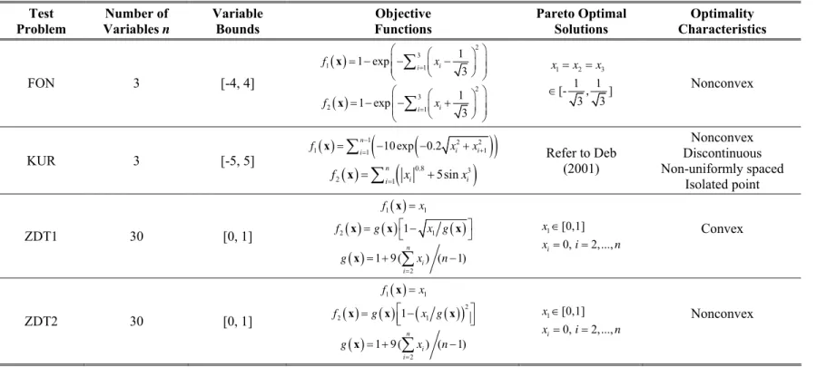
4.2. Benchmark Test Problems ... 62
4.3. MOEA Parameter Settings... 65
4.4. Performance Metrics... 66
4.4.1. Distance from the Pareto Optimal Front... 67
4.4.2. Diversity of Nondominated Solutions ... 67
4.4.3. Delineation of Pareto Optimal Front... 69
4.4.4. Hypervolume... 70
4.5. FPGA Computational Results... 71
4.5.1. Termination of the Search... 72
4.5.2. Discussion of the Results ... 74
4.5.3. A Discussion on FPGA Population Regulation... 82
CHAPTER 5 : PROPOSED METHODOLOGY FOR STOCHASTIC ENVIRONMENTS ... 85
5.1. Introduction... 85
5.2. Redefinition of Solution Dominance in Multiobjective Stochastic Environments 85 5.3. Noise ... 90
5.4. Stochastic Solution Ranking Strategy and Fitness Assignment ... 91
5.5. Sampling Operator ... 93
5.6. SPGA Computational Study ... 95
5.7. Discussion of Computational Results ... 98
5.7.3. ZDT4 Test Problem ... 104
5.7.4. ZDT6 Test Problem ... 104
CHAPTER 6 : SUMMARY AND FUTURE RESEARCH DIRECTIONS... 105
6.1. Introduction... 105
6.2. Summary and Conclusions ... 105
6.3. Future Research Directions... 107
6.3.1. Expanded Suite of Test Problems with Different Properties ... 107
6.3.2. Parameter Settings ... 108
6.3.3. Additional MOEA Performance Metrics ... 109
6.3.4. Statistical Comparative Analysis of Performance Metrics ... 110
6.3.5. Integration of the Proposed Methodology with Commercial Simulation Software 110 LIST OF REFERENCES... 111
LIST OF FIGURES
Figure 1.1: Illustration of strict dominance in a deterministic problem domain. ... 4
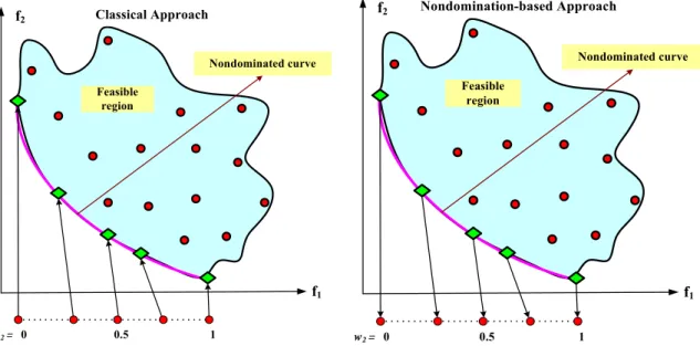
Figure 1.2: Illustration of the classical approach and nondomination-based approach for minimization problem with two objectives (Deb, 2001). ... 4
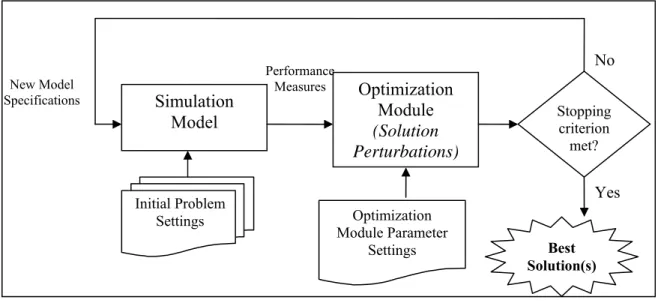
Figure 1.3: General process of simulation optimization... 6
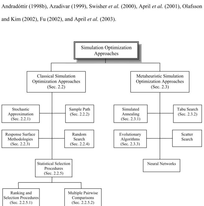
Figure 2.1. Taxonomy of existing simulation optimization approaches... 12
Figure 2.2. Flow diagram of NSGA (obtained from Srinivas and Deb (1994)). ... 37
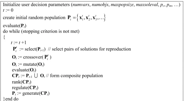
Figure 3.1. Pseudocode of the proposed fast Pareto genetic algorithm (FPGA). ... 47
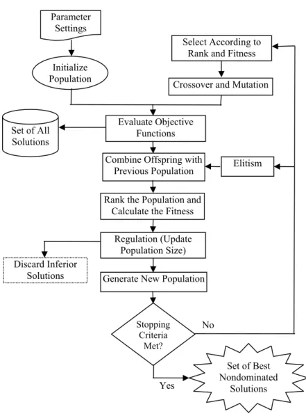
Figure 3.2. Logic flow of the fast Pareto genetic algorithm (FPGA). ... 48
Figure 3.3: Illustration of crowding distance calculation. ... 53
Figure 4.1.Diversity metric Δ... 69
Figure 4.2. Delineation metric Φ. ... 70
Figure 4.3. The velocity measure PPR on KUR... 73
Figure 4.4. The velocity measure PPR on ZDT6... 73
Figure 4.5. The populations with FPGA and NSGA-II on KUR... 77
Figure 4.6. The populations with FPGA and NSGA-II on ZDT1. ... 77
Figure 4.7.The populations with FPGA and NSGA-II on ZDT2. ... 78
Figure 4.8. The populations with FPGA and NSGA-II on ZDT3. ... 78
Figure 4.9. The populations with FPGA and NSGA-II on ZDT4. ... 79
Figure 4.10. The populations with FPGA and NSGA-II on ZDT6. ... 79
Figure 4.11. The populations with FPGA having poor diversity in few replications and NSGA-II on ZDT3... 81
Figure 4.12. Population regulation behavior of FPGA on ZDT6. ... 84
Figure 5.1. Plot of normally-distributed random variable t. ... 89
Figure 5.3. The populations with SPGA-s, SPGA-r and NSGA-II on ZDT1... 101 Figure 5.4. The populations with SPGA-s, SPGA-r and NSGA-II on ZDT4... 102 Figure 5.5. The populations with SPGA-s, SPGA-r and NSGA-II on ZDT6... 102
LIST OF TABLES
Table 2.1: Gradient estimation techniques for stochastic approximation (summarized from Fu (2002))... 15 Table 2.2. Commercial implementation of metaheuristic search strategies for simulation
optimization (obtained from Law and Kelton (2000))... 25 Table 2.3. Summary of simulation optimization approaches (obtained from Fu (2002)). 45 Table 4.1: Benchmark test problems. ... 63 Table 4.2: Parameter settings for FPGA and NSGA-II. ... 65 Table 4.3. Mean, standard deviation and 95% confidence interval of distance and
diversity metrics for FPGA and NSGA-II over the 30 random replications. ... 75 Table 4.4. Mean, standard deviation and 95% confidence interval of delineation Φ and
hypervolume ratio HVR metrics for FPGA and NSGA-II over the 30 random
replications... 76 Table 5.1: Parameter settings for SPGA and NSGA-II. ... 96 Table 5.2. Mean, standard deviation and 95% confidence interval of distance ϒand
diversity ∆metrics for SPGA-s, SPGA-r and NSGA-II over 50 random replications. ... 99 Table 5.3. Mean, standard deviation and 95% confidence interval of delineation Φ and
hypervolume ratio HVR metrics for SPGA-s, SPGA-r and NSGA-II over 50 random replications... 100
CHAPTER 1: INTRODUCTION
1.1. Multiobjective Optimization
In today’s competitive global business environment, a firm’s ability to make the most appropriate critical decisions can be translated into a great competitive advantage. Most of these critical decisions are multiple objective problems in which management should be able to handle the challenges of conflicting objectives. For example, in supply chain management, the objective of reducing total costs typically opposes the objective of decreasing lead times, and improving product quality. These conflicting objectives are also encountered in other problem settings including job shop scheduling, inventory control, facility location, portfolio management and project management. In recent years, multiple objective problems have begun to draw the attention of practitioners and academicians alike.
Several methods exist that one could use to solve problems involving multiple objectives (Szidarovszky et al., 1986; Mollaghasemi and Pet-Edwards, 1992). A naïve way is to select the most important performance objective and ignore the other less important objectives. This treatment of neglecting some objectives will undoubtedly result in poor solutions. Another method is to select a single objective for optimization and constrain the values of the other objectives to be within certain levels. The main drawback of this method is that the constrained objectives usually restrict the feasible solution space resulting in no feasible solution being found.
Other more traditional approaches for solving multiobjective optimization problems (MOPs) typically try to scalarize the multiple objectives into a single objective. This transforms the original multiple objective optimization problem formulation into a single objective optimization problem with a single solution. The major drawbacks of traditional methods that serve as motivation for using these alternative techniques include:
The priority (or weight) vector used in the scalarization process greatly influences the final solution;
Alternative solutions will not be available to decision-makers without at least changing some parameters such as the priority vector;
Some optimal solutions may never be found if the objective space is not convex for minimization problems (Szidarovszky et al., 1986 pp. 34-39); real-world problems are seldom convex (Silva and Biscaia, 2003);
There are implications in the homogenization of different performance measures (such as cost, quality of products, and cycle times) to a common unit of measure; and
Traditional approaches may not work effectively if objectives are noisy or have discontinuous variable space.
For example, consider the first drawback. A small perturbation in the priority vector values can greatly influence the obtained solution. Each certain pair of weights w1 and w2 (w2 = 1 – w1 for biobjective problem) results in single nondominated point in the tradeoff curve. However, the drawbacks of this class of approaches have motivated researchers and practitioners to seek alternative techniques to find a set of Pareto optimal
(nondominated) solutions rather than just a single solution (e.g., Srinivas and Deb 1994; Deb, 2001; Coello et al., 2002; Silva and Biscaia 2003). A solution is Pareto optimal if there exists no feasible solution for which an improvement in one objective does not lead to a simultaneous degradation in one or more of the remaining objectives.
1.2. Solution Dominance in Multiobjective (Deterministic) Problem Environments In deterministic problem environments, most multiobjective optimization applications are gravitating towards using the nondomination-based approaches due to the limitations of traditional multiobjective methods. Assume that fi(A) and fi(B) are the values of objective
function i (i ∈ {1, …, m}) for two solutions A and B, where A and B are p-dimensional vectors of the decision variables. The desire is to minimize each objective function. In a deterministic problem domain, solution A strictly dominates (is better than) solution B if fi(A) is less than fi(B) for each objective function i. Figure 1.1 illustrates the concept of
strict dominance graphically for an optimization problem in which m = 2 and the goal is to minimize both functions f1 and f2. In the figure, it can be seen that solution A strictly dominates all solutions in the shaded region, including solution B. It must be noted that in stochastic problem environments where the objective function values are uncertain, the definition of strict solution dominance must be modified. Nondomination considers all possible tradeoffs of the priorities of the given objectives, as shown in Figure 1.2, which shows the problem of minimizing two objectives.
Solution A strictly dominates all solutions in the shaded region
f2 Minimize Mi ni miz e A f1 B
Figure 1.1: Illustration of strict dominance in a deterministic problem domain.
f2 f1 Nondomination-based Approach f2 f1 Classical Approach Nondominated curve Nondominated curve
Figure 1.2: Illustration of the classical approach and nondomination-based approach for minimization problem with two objectives (Deb, 2001).
1.3. Systems Simulation Modeling
Due to the complexities and uncertainties existing in real-world problems, it is very difficult to solve single objective problems, let alone multiobjective problems, exactly using traditional analytical models. As an alternative to analytical methods,
Feasible region Feasible region 0 0.5 1 w2 = 0 0.5 1 w2 =
computer simulation is an effective approach that can be used to model the complexities and uncertainties of the real-world problems without the limiting assumptions. Simulation can estimate the measures of the system performance. This is accomplished by performing n simulation replications. It is appropriate to note here that a known drawback of using simulation is that it can be computationally-expensive and time-consuming. When simulating realistic, large-scale stochastic systems, even a single replication can be computationally-prohibitive. Each replication is one sample observation (point estimate) for the performance measure. Then, the arithmetic mean of the n independent and identically distributed sample observations is used as an unbiased point estimate of the true population mean. Due to the randomness in the simulation model, a confidence interval is usually constructed for each system performance measure of interest. The analyst asserts that this confidence interval contains the true mean with a certain level of confidence. In most simulation studies, confidence intervals are employed in the output analysis of the model in addition to the sample means.
However, simulation modeling facilitates policy evaluation of a system and “what if” analyses. It alone lacks optimizing ability, and thus, should be combined with other analysis techniques to become most effective for optimization problems. The general approach to address this problem is the integration of an optimization subroutine or module with the simulation model.
1.4. Optimization via Simulation
In general, simulation optimization is the process of searching for the best set of model specifications, i.e., input parameters and structural assumptions, where the
(Olafsson and Kim, 2002). Figure 1.3 shows the general process of optimization via simulation. The optimization module uses the numerical values of the performance measures estimated by a simulation model (or set of models) to make decisions regarding the next set of candidate solutions. Thereafter, the optimization algorithm generates new model specifications through perturbations of existing solutions that are fed to the simulation model. This search continues until a user-specified stopping criterion is satisfied. Simulation Model Optimization Module (Solution Perturbations) Stopping criterion met? Initial Problem Settings No Yes Performance Measures New Model Specifications Best Solution(s) Optimization Module Parameter Settings
Figure 1.3: General process of simulation optimization.
Several simulation optimization approaches have been proposed by researchers. They differ primarily based on the problem settings and characteristics. Such settings and characteristics for simulation optimization problems include the nature of the solution space (continuous or discrete decision parameters), number of feasible solutions (relatively small, large but finite, or countably infinite), number of the performance measures (single objective or multiple objectives) (Andradóttir, 1998b; Azadivar, 1999; Swisher et al., 2000; Olafsson and Kim, 2002). . It is also worthy to note that there is a
considerable gap between the approaches proposed in the research literature and those that are employed by commercial software packages for practical use.
Since evaluation of the measures of the system performance is performed by executing simulation runs that are often computationally-expensive and time-consuming, it is very important that an optimization algorithm be able to find optimal or near-optimal solutions in the early stages of the search process. The optimization algorithm should also be capable of effectively balancing the tradeoff between solution space exploration and solution space exploitation. In other words, an intelligent algorithm should search the feasible solution space thoroughly, and evaluate the regions around the local optima carefully in order to possibly find global optimal solution, which may be in another region. On the other hand, an optimization algorithm should be robust enough to handle the challenges of randomness and uncertainty involved in the estimated objective functions of the simulated model. In this case, the existing uncertainty and noise might hinder the optimization algorithm trying to move into improving directions.
1.5. Simulation Optimization of Multiple Stochastic Objectives
An issue that should be considered in the stochastic optimization context is the randomness effect of conflicting performance measures in the simulation models caused by the uncertain nature of different processes of the underlying system. The randomness effect of the performance measures plays an important role in the quality of the obtained results; thus, inefficient methods may lead to incorrect conclusions and improper decisions. The stochastic nature of simulation models together with costly simulation experimental runs makes the efficiency of the optimization methodology critical.
Due to the complexity and difficulty of dealing with these kinds of problems, few attempts have been made in multiobjective simulation optimization. The majority of these works focus on utility theory, interactive approaches, response surface methodology and goal programming (Mollaghasemi, 1994; Boyle and Shin, 1996; Lee et al., 1996; Baesler and Sepulveda, 2000). To the best of the author’s knowledge, the existing literature does not support an efficient approach for multiobjective simulation optimization to find Pareto optimal solutions.
1.6. Objectives of This Research
The primary objective of this study is to provide a modeling framework that integrates simulation models and nondomination-based multiobjective optimization methods. More specifically, in many applications of simulation modeling, the time to perform a single solution evaluation (replication) is of the order of minutes to hours, restricting the total number of solution evaluations needed for statistical precision. Additionally, many real-world problems often involve complicated stochastic (or noisy) multiple objective functions making a large number of the necessary replications computationally-prohibitive. Therefore, a multiobjective optimization algorithm capable of finding diverse Pareto optimal solutions and handling the uncertainty of stochastic multiple objective functions would be greatly beneficial. The purpose of this research is to propose such a stochastic multiobjective optimization methodology that finds evenly-distributed Pareto optimal solutions in a computationally-efficient manner.
1.7. Contributions of This Research
This research proposes two new multiobjective evolutionary algorithms (MOEAs), called fast Pareto genetic algorithm (FPGA) and stochastic Pareto genetic algorithm (SPGA), for optimization problems with multiple deterministic objectives and stochastic objectives, respectively.
New concepts of solution dominance are defined for better discrimination among competing solutions in stochastic environments. SPGA uses a solution ranking strategy based on these new concepts.
New genetic operators are introduced to enhance both algorithms’ performance in finding Pareto optimal solutions while minimizing computational effort. An elitism operator with high intensity is employed to ensure the quick propagation of the nondominated solutions, and a dynamic regulation operator to dynamically adapt the population size.
In addition to distance and hypervolume ratio metrics, two new metrics, called diversity and delineation, are suggested to better discriminate among the MOEAs. New stopping criterion is introduced in which different numbers of solution
evaluations are used for different test problems depending on the complexity of the problem.
1.8. Organization of This Dissertation
The remainder of this document is organized as follows. CHAPTER 2 briefly a reviews the existing literature in the area of simulation optimization. CHAPTER 3 presents the proposed framework for solving multiobjective simulation optimization problems. After introducing new solution dominance concepts for stochastic problem
which uses an evolutionary algorithm, is discussed. CHAPTER 4 summarizes the performance of the proposed framework for deterministic problem environments. It first discusses the experimental design followed by the computational results, including the comparison of the proposed methodology with another state-of-the-art algorithm to assess its performance. CHAPTER 5 discusses an enhancement of the proposed framework that makes it appropriate for stochastic problem environments. New dominance concepts are presented. Experimental results show the enhanced approach’s competitiveness against a well-known state-of-the-art algorithm. This dissertation is concluded in CHAPTER 6 with a summary of the research and proposed directions for future study.
CHAPTER 2: OVERVIEW OF SIMULATION OPTIMIZATION THEORY AND APPROACHES
2.1. Introduction
In general, simulation optimization is the process of finding the best values of a set of decision variables, where the objective value is the output performance of simulation model for the underlying system. More specifically, in simulation optimization, one tries to find the best system design or solution to optimize the objective function
( )
min / max f
θ∈Θ θ , 2.1
where θ denotes a k-dimensional vector of decision variables of the system, Θ represents the constraint set on θ (feasible region), and f(θ) is the real objective function, representing the expected system performance. There is no explicit analytical expression for the objective function f when f is stochastic, or it is very complicated if available (Law and Kelton, 2000, p. 646). Typically, this objective function is estimated using a function of the stochastic output X(θ), which might be an unbiased estimate for f(θ); that is, f(θ) = E[X(θ)] (Olafsson and Kim, 2002). There are other ways of formulating the simulation optimization problem. They can be found in Azadivar (1999).
Sections 2.2 and 2.3 present a brief review and several advantages, disadvantages, and applications of several simulation optimization techniques. Figure 2.1 shows the most popular simulation optimization approaches as categorized in this literature study. There are other ways to categorize simulation optimization approaches based on the
nature of the search space, e.g., continuous decision variables versus discrete decision variables. Further material in this regard can be found in Fu (1994), Andradóttir (1998a), Andradóttir (1998b), Azadivar (1999), Swisher et al. (2000), April et al. (2001), Olafsson and Kim (2002), Fu (2002), and April et al. (2003).
Simulation Optimization Approaches Classical Simulation Optimization Approaches (Sec. 2.2) Metaheuristic Simulation Optimization Approaches (Sec. 2.3) Stochastic Approximation (Sec. 2.2.1) Response Surface Methodologies (Sec. 2.2.3) Sample Path (Sec. 2.2.2) Random Search (Sec. 2.2.4) Statistical Selection Procedures (Sec. 2.2.5) Multiple Pairwise Comparisons (Sec. 2.2.5.2) Ranking and Selection Procedures (Sec. 2.2.5.1) Simulated Annealing (Sec. 2.3.1) Evolutionary Algorithms (Sec. 2.3.3) Tabu Search (Sec. 2.3.2) Scatter Search Neural Networks
2.2. Classical Approaches for Simulation Optimization
Fu (2002) reports that research of classical approaches for simulation optimization includes five different categories:
1) stochastic approximation (i.e., gradient-based approaches); 2) sample path optimization (also known as stochastic counterpart); 3) (sequential) response surface methodologies;
4) random search; and
5) statistical selection approaches (ranking and selection, multiple pairwise comparison).
2.2.1. Stochastic Approximation
Stochastic approximation (SA) is an iterative process that attempts to mimic the gradient search method used in deterministic optimization. The best known stochastic approximation algorithms are first introduced by Robbins and Monro (1951) and Keifer and Wolfowitz (1952). The general stochastic approximation methodology is based on the equality
( )
(
)
1 ˆ n+ = Πθ n− ∇an f θ θ θn , 2.2where ˆ
( )
is the estimate of the gradient, nf
∇ θ Πθ denotes some projection back into the
feasible region and an is the step size at iteration n. Under certain conditions, when the
step size approaches zero with an slow enough rate, the asymptotic convergence of the SA algorithm can be guaranteed, i.e., limn→∞ an = 0, and ∑n an = ∞ according to the
SA-based algorithms are generally used in simulation optimization problems with continuous decision variables. However, SA has also been applied to discrete variable problems (see, for example, Gerencser (1999)). Some of the major drawbacks of this approach are its slow convergence rate, its lack of an appropriate stopping rule and its difficulty in handling constraints (Shapiro, 1996). It has been found that, in practice, the performance of a SA-based algorithm strongly depends on the choice of the step size (Fu, 2002). Another disadvantage of this method is that it might find local optima, since it is based on gradient search method.
Many gradient estimation techniques have been developed to estimate the gradient in Eq. 2.2. One way for estimating the gradient in this equation is using either the naïve one-sided finite differences (FD) or two-sided symmetric differences (SD) given as
( )
ˆ(
)
ˆ( )
ˆ n n i n i n f c e f g c + − = θ θ θ , and 2.3( )
ˆ(
)
ˆ(
)
ˆ 2 n n i n n i i n f c e f c e g c + − − = θ θ θ , 2.4respectively, where ei denotes the unit vector in the ith direction and cn represents a small
change in each decision variable. One-sided finite differences and two-sided symmetric differences need k+1 and 2k simulation replications (k is the dimension of the vector θ) respectively, which require considerable computational effort. Spall (1992) proposes the simultaneous perturbations (SP) technique in order to increase computational efficiency. This technique, which perturbs the solution in all directions simultaneously, requires only two simulation replications regardless of the dimension of the search space. Spall (1992)
shows that the asymptotic convergence rate of the simultaneous perturbations is the same as that of the FD technique.
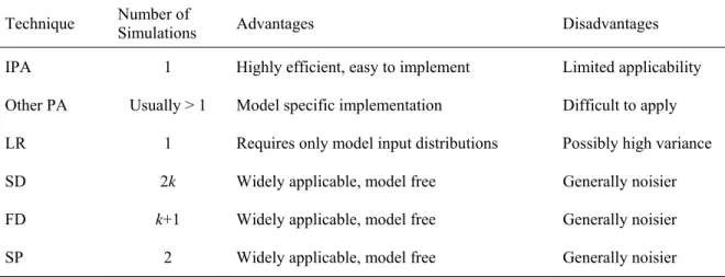
In order to improve the computational effort and convergence rate of the SA technique, many researchers focus on the direct estimation of the gradient. The best known techniques for direct gradient estimation are perturbation analysis (PA) (Glasserman, 1991; Ho and Cao, 1991) and likelihood ratio (LR) (Rubinstein, 1991; Rubinstein and Shapiro, 1993). Infinitesimal perturbation analysis (IPA) is a widely-used variant of the PA techniques. Kapuscinski and Taylor (1999) report that they successfully use IPA for optimization of capacitated production inventory systems. Fu (2002) summarizes the advantages and disadvantages of the main gradient estimation techniques, as shown in Table 2.1.
Table 2.1: Gradient estimation techniques for stochastic approximation (summarized from Fu (2002)).
Technique Number of Simulations Advantages Disadvantages
IPA 1 Highly efficient, easy to implement Limited applicability Other PA Usually > 1 Model specific implementation Difficult to apply LR 1 Requires only model input distributions Possibly high variance SD 2k Widely applicable, model free Generally noisier
FD k+1 Widely applicable, model free Generally noisier
SP 2 Widely applicable, model free Generally noisier
2.2.2. Sample Path Optimization
Sample path optimization includes methods that attempt to approximate the original simulation optimization problem with a set of deterministic continuous optimization problems. To demonstrate the framework, suppose that Y1, …, YN are N
independent random variables, where N is the size of the sample path (simulation replication), and a function h such that Xi(θ) = h(θ,Yi) has the cumulative distribution
function Fθ for i = 1, …, N. Then, the objective function is approximated by the sample mean over the N sample paths as
( )
1 1 ˆ N ( , ), for all N i i f h Y N = =
∑
∈ θ θ θ Θ. If each of theh(θ,Yi) are independent and identically-distributed (IID) unbiased estimates of f(θ), then,
for a sufficiently large N, the deterministic objective function approximates the expected objective function of the original simulation problem (Andradóttir, 1998b). In the simulation context, the common random numbers (CRNs) variance reduction technique provides the same sample path to calculate over different values of θ.
( )
ˆ N f θ( )
ˆ N f θ( )
ˆ N f θThe main advantage of the sample path optimization methodology relative to gradient-based methods is that it is capable of handling optimization problems with complicated constraints (Fu, 2002). Rubinstein and Shapiro (1993) introduce the stochastic counterpart (SC) method, a variant of the sample path optimization method, to overcome the slow convergence rate, lack of robust stopping rule, and difficulties for handling constraints characteristic of SA-based methodologies. In this approach, f(θ) is approximated using the likelihood ratio method.
2.2.3. Response Surface Methodology
Generally, response surface methodology (RSM) is based on the principle of building metamodels that attempt to obtain an approximate functional relationship between the input decision variables and output objective function. RSM attempts to fit a
polynomial of appropriate degree to the response surface formed by different input decision variables. There is a variety of metamodeling approaches, and the two best known approaches are regression models and neural networks. Other metamodeling approaches include multivariate adaptive regression splines, radial basis functions, frequency domain approximations, spatial correlation models, and interpolative models known as kriging. Detailed discussions of these types of metamodels can be found in Barton (1998).
In the most recent research literature, metamodeling is performed in a more localized way called sequential response surface methodology, or sequential metamodeling. Sequential RSM procedures avoid exploring the entire search space, which can be costly and often impractical. Rather, it employs linear polynomials to approximate the response surface in small sub-regions of the feasible region. Thereafter, the gradient estimation and steepest decent method is used to move to a new sub-region. This exploration process continues until the linear model becomes inadequate as indicated by the approximated response surface with slope of zero. This implies that the sub-region includes the optimal point and higher order of response surface is required for appropriate fitness. Canonical and ridge analysis is usually employed to examine this sub-region thoroughly with regression models.
Safizadeh (2002) shows that, under certain conditions, the smaller size of the RSM sub-region reduces both the bias and variance of the gradient estimate. He provides guidelines for manipulating the size of the sub-region. In the study, a strong assumption is made that the positive correlation between the performance measures of two simulation
replications decreases when the difference of the values of input decision variables increases.
Keys and Rees (2004) propose a new sequential metamodeling strategy based on the nonparametric thin-plate splines. In their proposed procedure, the exploration starts with a uniform grid of points, and then the location of next system design point is found from the solution of a mathematical programming model. This solution is based on the distribution of the quantiles of estimated second derivatives of the response function.
It is worthy to note that even sequential RSMs require a substantial amount of computational effort, particularly when the number of decision variables is large. If the response surface of any sub-region has multiple optima, then the linear polynomial is not necessarily a good approximate. To obtain a better approximate, replications with a smaller sub-region is required to provide more accurate information. This problem makes the search for optimal solutions dramatically slow and increases the computational time.
2.2.4. Random Search Method
Random search method typically involves an iterative process in which the search moves successively from the current solution to a randomly-selected new (possibly better) solution in the neighborhood of that solution. This implies that the neighborhood structure must be well-connected in a certain precise mathematical sense so that the search may converge for all initial solutions (Andradóttir, 1998b). Random search methods have been mainly used for discrete variable optimization problems, though there is no particular theoretical reason that prevents applying them to continuous optimization problems. Random search methods are of special appeal for their generality and existence
of theoretical convergence proofs (Fu, 2002). The general random search, also summarized by Olaffson and Kim (2002), is as follows:
(0) Set iteration index i = 0; Select an initial solution θi and perform the simulation to
obtain expected value X(θi).
(1) Select a candidate solution θcfrom the neighborhood of the current solution N(θi)
according to some pre-specified probability distribution and perform the simulation to obtain expected value X(θc).
(2) If the candidate satisfies the acceptance criterion based on the simulated performance, then θi+1 = θc; otherwise θi+1 = θi.
(3) If the termination criterion is satisfied, then terminate the search; otherwise i = i+1 and go back to Step 1.
Different random search methods found in the literature primarily vary in the choice of the neighborhood structure, the method of candidate selection, the acceptance and termination criteria (Olafsson and Kim, 2002). The best known variants of the random search methods are the stochastic ruler algorithms, originally proposed by Yan and Mukai (1992), and those based on the simulated annealing approach. Detailed discussions on random search methods can be found in Andradóttir (1998b).
2.2.5. Statistical Selection Procedures
Statistical selection procedures are designed to distinguish the best solution(s) from among a given finite set of feasible solutions, that is Θ=
{
θ θ1, ,2 K,θn}
, where n is relatively small. In the simulation context, statistical analysis is required to evaluate each feasible solution and compare their performance measure in order to consider uncertaintysurrounding the stochastic output. Several statistical procedures have been developed including ranking and selection (R&S) procedures and multiple pairwise comparison (MPC) procedures to address this problem. The primary difference between these two classes of procedures is that R&S procedures ensure the correct selection of the best solutions thar are within user-specified confidence and precision levels. MPC procedures make certain pairwise comparisons among feasible solutions in order to provide some inferences in the form of confidence intervals. In other words, R&S procedures help the analyst make a decision, whereas the latter only provide some statistical inferences for system performance between each pair of system design alternatives. A brief review of commonly used statistical selection procedures is now given.
2.2.5.1. Ranking and Selection
Ranking and selection is a practical tool for selecting the best solutions among a given set of competing solutions. The most popular R&S method is indifference zone ranking and selection. Assuming that decision-makers are indifferent to performance measure differences less than precision level δ > 0, one can follow a procedure to make the right selection with a certain probability of correct selection, P*. In other words, with
at least a certain probability P*the performance of the selected solution θ’ is within the δ
interval of the performance of the best solution θ*
( )
( )
(
')
*Prob | f θ − f θ* |< ≥δ P . 2.5
The precision level δ is called the indifference zone and probability of correct selection P* is actually confidence level (1-α), and both should be pre-specified by the user. The two-stage procedure developed by Dudewicz and Dalal (1975) estimates the
appropriate number of simulation replications in order to guarantee the desired confidence of correct selection. In the first stage of sampling, the means and variances of each of the n feasible solutions are evaluated using r0 ≥ 2 replications. Then, the variances obtained in the first stage are used to determine the number of additional replications required for each solution in the second stage, say ri (i = 1, …, n).
Specifically,
( )
2 2 0 0 2 max 1, i i h S r r r δ ⎧ ⎡ ⎤⎫ ⎪ ⎪ = ⎨ + ⎢ ⎥⎬ ⎪ ⎢ ⎥⎪ ⎩ ⎭, 2.6where ⎡ ⎤⎢ ⎥x is the smallest integer that is greater than or equal to the real number x, and h is a constant that depends on r, P*, and δ, which can be found in a given table. Finally,
the weighted sample means is estimated and the best solution is selected. Intuitively, the higher confidence level P*, or the more precision level (the smaller δ), the more
replications is required which corresponds to Eq. 2.6. Values for P* and δ should be
selected depending on the goal of study and the system of interest (Law and Kelton, 2000). The initial number of replications r0 plays an important role in determining the required computational time of the underlying system. It is advised that r0 be at least 20 so that poor first stage variances are minimized, which usually results in a large number of required additional replications.
Ranking and selection procedures are easy to implement and interpret. This makes them popular when the number of system design alternatives n are relatively small, i.e., 2 to 20. However, when the number of design alternatives is quite large, these procedures are inefficient and even impractical in terms of computation time. The reason is: (1) in Eq. 2.6, the constant h is an increasing function of n, and (2) Eq. 2.6 is derived based on
the worse case scenario, which means that the best design is exactly δ better than the other (n-1) system designs, which are all viewed as the second best designs. Thus, when the number of alternatives is large, a great amount of computational effort is required for the inferior alternatives making the analysis quite time-consuming and maybe computationally-prohibitive. Nelson et al. (2001) address this problem by proposing procedures for selecting the best design alternative, and they argue that these procedures are statistically more efficient than conventional procedures. They use the data provided in the first stage sampling to screen out the inferior alternatives, and the second stage sampling, which usually requires more computational effort, only includes the superior alternatives.
Another R&S procedure called subset selection attempts to find a subset of alternatives containing the best system design to screen out the inferior alternatives. This approach is useful when specification of several good alternatives is desired in the sense that the best alternative might be rejected for any reason. The first subset selection procedure is suggested by Gupta (1956) in which a random size subset containing the best design alternative is selected with user specified correct selection P*, and without
any indifference zone specification, i.e., δ = 0. This original procedure requires the assumptions of normality and equal and known variances among alternatives that are rarely satisfied in simulation optimization problems. Koenig and Law (1985) develop the indifference zone procedure, suggested earlier by Dudewicz and Dalal (1975), for R&S problems in application of selecting a subset of the given size m containing the best of n alternatives. The only difference between these two is that the indifference zone subset selection procedure takes on different values of h depending on m, n, δ,and P*. However,
it is reported in the literature that the goal of most simulation studies is to specify the best system design rather than produce a subset of designs containing the best (Swisher and Jacobson, 1999).
2.2.5.2. Multiple Pairwise Comparisons
The main goal of the multiple pairwise comparison (MPC) procedures is to gain some statistical insight in the form of confidence intervals about the differences of each pair of design alternatives without guaranteeing any decision. There are several types of MPC procedures, including paired-t, Bonferroni, all-pairwise comparisons, all-pairwise multiple comparison (MCA), multiple comparison with a control (MCC), and multiple comparison with the best (MCB) (Swisher and Jacobson, 1999).
In paired-t, Bonferroni and all-pairwise multiple comparison (also called brute force), all possible pairwise comparison are performed constructing confidence interval for n system design alternatives. Using the Bonferroni approach, n(n-1)/2 confidence intervals are constructed at the confidence level of
(
1−α ⎡⎣n n(
−1)
2⎤⎦)
in order to provide the overall confidence level of (1-α) for all intervals simultaneously. This method is useful when the number of alternatives is quite small; otherwise, individual confidence intervals become wide and do not provide useful inferences. MCA methods are similar to the brute force approach except it constructs a simultaneous set of confidence intervals with the same half-width at an overall confidence level of (1-α). MCC techniques are typically used in the case when the analyst wishes to compare a set of design alternatives to a pre-specified system design such as to an existing design. The MCB approach is the most popular MPC procedure that attempts to identify the bestdesign from a set of alternatives. It requires constructing only n-1 simultaneous confidence intervals as μ minμ
≠ − i
i j j for i = 1, 2, …, n, which is significantly less than those of the brute force approach.
Applying MCA, MCC, or MCB procedures requires IID with (approximately) normal distributions as well as equal variances. Yang and Nelson (1991) consider this requirement and modify MCA, MCC, and MCB procedures by incorporating two variance reduction techniques – common random numbers and control variates. They report that using variance reduction techniques achieves better statistical precision and ensures more confident decisions.
2.3. Metaheuristic Search Approaches for Simulation Optimization
Metaheuristic approaches have drawn considerable attention from many researchers in the last decade. The most popular metaheuristics are simulated annealing, tabu search, evolutionary algorithms, scatter search and neural networks. Each of these search heuristics has its own set of search features that makes them capable of escaping local optima. These approaches are all considered global search strategies in that they are capable of find optimal or near-optimal solutions in relatively short amounts of time. Originally designed for combinatorial optimization problems in the deterministic environment, these methods have been adapted for the stochastic environment associated with discrete simulation optimization, and they have been successfully applied to many real-world simulation problems.
It is important to note that several commercial software implementations currently incorporate these metaheuristic approaches. Although classical approaches for simulation
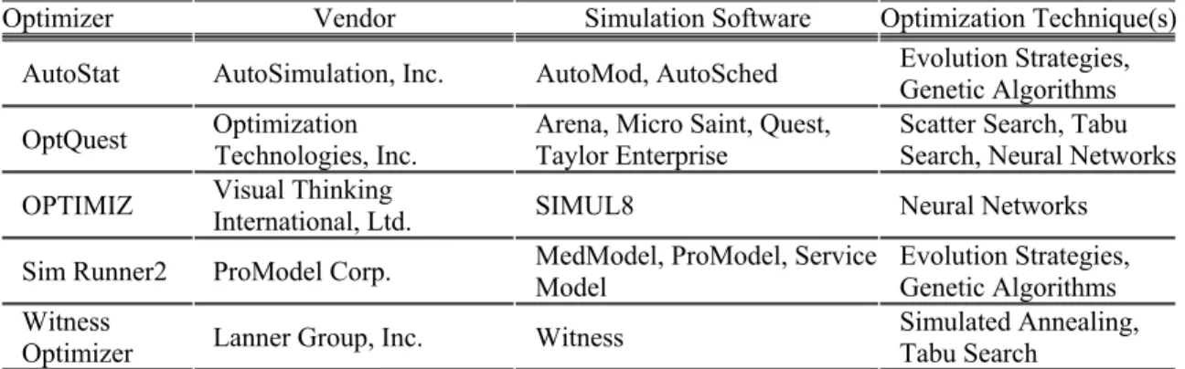
optimization account for a substantial amount of the research literature, none of them have been used in optimization modules embedded in the available commercial simulation software packages. Law and Kelton (2000) summarize the optimization methodologies utilized in the more popular commercial packages. This summary is given in Table 2.2. A brief discussion of the three best known metaheuristics follow. These are simulated annealing, tabu search and evolutionary algorithms.
Table 2.2. Commercial implementation of metaheuristic search strategies for simulation optimization (obtained from Law and Kelton (2000)).
Optimizer Vendor Simulation Software Optimization Technique(s) AutoStat AutoSimulation, Inc. AutoMod, AutoSched Evolution Strategies, Genetic Algorithms OptQuest Optimization Technologies, Inc. Arena, Micro Saint, Quest, Taylor Enterprise Scatter Search, Tabu Search, Neural Networks
OPTIMIZ Visual Thinking International, Ltd. SIMUL8 Neural Networks Sim Runner2 ProModel Corp. MedModel, ProModel, Service Model Evolution Strategies, Genetic Algorithms
Witness
Optimizer Lanner Group, Inc. Witness Simulated Annealing, Tabu Search 2.3.1. Simulated Annealing
Simulated annealing is a random local search technique that mimics the physical annealing process for crystalline solids. In this process, the molten solid is cooled very slowly from a high temperature until it reaches the ground temperature with a low energy state. If the cooling process occurs too quickly, the crystal is trapped in a much higher energy state than that of perfect crystal. In this analogy, state, energy, ground state, rapid quenching, temperature and careful annealing in the physical system correspond to feasible solution, evaluation function, optimal solution, local search, control temperature parameter and simulated annealing in the optimization problem (Michalewicz and Fogel, 2000).
In this method, search starts from an initial solution and moves from one solution to the candidate solution from its neighborhood, which is randomly selected. In order to overcome being trapped at local optima, simulated annealing allows acceptance (with certain probability) of inferior candidate solutions, or (for minimization problem)
(
)
( ) ( )( )
( )
1, if Prob Accept , otherwise C i i C i X X C T X X e − < ⎧ ⎪ = ⎨ ⎪⎩ θ θ θ θ θ , 2.7where Ti is the temperature parameter at iteration i that usually decreases during the run.
This means that the candidate solution is certainly accepted if it is superior to the current solution. Otherwise, it is accepted with certain probability at which higher difference in their performance makes it less likely of accepting new solution. Simulated annealing is generally different from stochastic hill climbing only in temperature parameter, which is kept fixed in the latter method (Michalewicz and Fogel, 2000). The search usually starts with high values of T, and then it gradually decreases when the search progresses according to a function commonly referred to as the cooling, or annealing, schedule. This implies that the procedure starts with purely random search and ends in ordinary hill climbing approach with the hope of not being trapped at a local optimum and converging to the global optimum. Various cooling schedules have been proposed in the literature, including monotonic schedules, geometric schedules, and adaptive schedules. Alrefaei and Andradóttir (1999) report that they successfully use a constant temperature parameter in a specific simulation optimization problem.
The main advantage of simulated annealing relative to other metaheuristic approaches is that it has been shown to guarantee convergence in many settings (Jeon and Kim, 2004). On the other hand, it requires excessive computation time in practice, and it
is relatively slow in converging to good solutions in comparison to other metaheuristic approaches. Further, simulated annealing cannot perform intensification and diversification in an efficient manner (Jeon and Kim, 2004). Intensification reinforces attributes historically found good in order to return towards attractive regions to explore them carefully, while diversification drives the search into perhaps more promising regions.
Many different variants of simulated annealing have been suggested within the last decade in order to improve the drawbacks of the conventional version. For example, Azizi and Zolfagari (2004) propose two variations of the simulated annealing algorithm and successfully use them to minimize the makespan of a set of n jobs in the job shop scheduling problem. They note in their work that if some local optima are located at the relatively low temperature towards the end of the search, the search becomes trapped at a local optimum and the global optimal solution cannot be obtained. In their first approach, called adaptive simulated annealing, they consider the characteristics of the search trajectory in which adaptive cooling schedule is used that adjusts the temperature dynamically based on the number of consecutive improving moves. In this adaptive cooling schedule, the temperature is controlled by a single function at which temperature is kept above a minimum level. The temperature increases when any uphill move occurs. Such an improvement addresses the limitation of the traditional simulated annealing algorithm of having significantly low transition probability toward the end of the search.
2.3.2. Tabu Search
memory-forbidding (or penalizing) moves that take a solution located in the previously visited region of the search space. The main idea of tabu search is that the memory enforces the search to deeply explore new areas of the search space within a single execution. The search keeps track of the sequence of recent moves or visited solutions in a memory list. A standard form of tabu list records the solutions that have been visited in the n last moves, where n is the tabu tenure. The best solution located in the neighborhood of the current solution is selected as the candidate solution if this move is not forbidden (i.e., not in the tabu list). If this move is forbidden, the next best candidate solution from the neighborhood is selected that is not classified as tabu. However, in order to avoid not selecting a superior tabu solution found during the search, the tabu classification can be overridden when a predetermined aspiration criterion is satisfied. One popular aspiration criterion is to select the tabu move if it is the best ever solution found in the search that has not been visited before (Ho and Haugland, 2004). Finally, as with all metaheuristic search techniques, a stopping criterion determines when the search process halts. Usually, the search stops when a prespecified number of iterations has been completed, or when the current best solution has not been improved above a specified percentage within a certain number of consecutive iterations.
The type of memory described above is called short-term memory, or recency-based memory. Another type of memory, called frequency-recency-based memory, or long-term memory, encourages moves that have led to solutions whose attribute have rarely been seen before (diversification). It also encourages moves that have historically led to improvements by reinforcing the consideration of special attributes of previously found good solutions in the remaining exploration (intensification) (Glover et al., 1999). For
instance, long-term memory may allow the search to restart from a previously seen good solution with a different tabu list that guides the search in another direction from the good initial solution (Olafsson and Kim, 2002). One popular approach for long-term memory implementation is to measure the absolute frequency of a selected move during the search. An efficient implementation of long-term memory can balance between the diversification and intensification functions and increase the performance of the algorithm considerably.
Tabu search is a deterministic search approach and cannot guarantee the convergence. However, exploitation of the adaptive memory strategy is the unique feature of this search method that distinguishes it from other metaheuristic approaches. Many researchers have recently incorporated the adaptive memory feature of tabu method in their proposed metaheuristic algorithms. For example, Azizi and Zolfaghari (2004) incorporate a tabu list to their adaptive simulated annealing algorithm in order to improve the performance of their methodology by taking advantage of the tabu memory structure in order to keep track of recently visited solutions and prevent cycling. It has been reported that the combination of the tabu method with the complementary population-based approach of scatter search is a considerably powerful tool for simulation optimization problems (Glover et al., 1999). Factors that affect the performance of tabu search include proper appropriate selection of the neighbor of a solution, the number of moves classified as tabu in the memory list, proper combination and management of the short-term and long-term memory, and efficient implementation of the intensification and diversification mechanisms (Jeon and Kim, 2004).
Tabu search has been widely used in a variety of applications ranging from job shop scheduling to power systems. For instance, Ho and Haugland (2004) use a tabu search algorithm to solve the vehicle routing problem with time windows and split deliveries. Time windows means that each customer has their own time interval in which to receive the service, and split deliveries means that the demand of a customer may be met by more than one vehicle, when the demand size exceeds the vehicle capacity. They apply tabu search successfully to minimize the number of vehicles, and the total distance traveled. They use a unique neighborhood structure that is defined by a union of four move operators including relocate, exchange, 2-opt, and relocate split operators.
2.3.3. Evolutionary Algorithms
Evolutionary algorithms are nature-inspired heuristics based on the Darwinian evolution theory on survival of the fittest (Holland, 1975; Goldberg, 1989; Mitchell, 1996). The main idea behind this family of algorithms is a population of individuals (solutions) with certain attributes is exposed to an environment. Some of the individuals are better suited to satisfy the requirement of the environment (i.e., survive) and thus have more chance to be selected for populating the next generation of solutions. Their attributes are inherited by their offspring in the next generation. As a consequence, over several generations, inferior individuals with undesired attributes are gradually eliminated and the superior individuals evolve and eventually dominate the population. Such evolution is accomplished through different biological reproduction operations on the current individuals (parents) to generate the offspring for the new population. The most common operators include crossover and mutation. The crossover operator typically
more chance to be selected) and combine them to make two new individuals. Thereafter, the mutation operator takes each individual and changes it slightly.
Evolutionary algorithms have many advantages over classical optimization approaches. One of the main advantages is that it is a population-based approach, which implies that if an optimization problem has multiple optimal solutions, an evolutionary algorithm is capable of finding multiple optimal solutions in its final population, whereas a classical optimization approach may find only a single optimal solution.
Another advantage of evolutionary approaches over those based on the locally searching the neighborhood of each single solution is their capability of more thoroughly exploring the feasible solution space in an efficient manner in terms of computational time (April et al., 2003). The performance of the local search approaches based on the neighborhood sampling strongly depends on the distance of the optimal solution from the starting point as well as the appropriate definition of neighborhood because move operations can direct the search towards the optimal solution. Given the fact that in the stochastic simulation optimization context the fitness functions are estimated by running the expensive simulation models, finding a near-optimal or even good solution in an acceptable short period is considerably preferential.
Lacksonen (2001) performs an empirical study to compare the Hooke-Jeeve pattern search, Nelder-Mead simplex, simulated annealing, and genetic algorithm optimization approaches on variations of four industrial case study simulation models with 25 different test problems. Combinations of real variables, integer variables, non-numeric variables, deterministic constraints, and stochastic constraints are considered in the test problems. Based upon the general results regarding solution quality, the
decreasing order of the optimization approaches in terms of robustness of performance is genetic algorithms, pattern search, simulated annealing and simplex method. Genetic algorithms are found to be the most robust approach, since it finds near optimal solutions for all 25 test problems. The pattern search appears to be robust for small and medium size problems (less than 12 variables) with numeric variables. Simulated annealing and the simplex method are not found to be very robust approaches. However, it is important to note that these results are based on only 25 test problems in four application areas, and the performance of the approaches might be different on other test problems.
2.4. Evolutionary Algorithms for Multiobjective Optimization
As previously mentioned, evolutionary algorithms (EAs) are population-based search algorithms inspired by Darwinian evolutionary theory. It has been shown that EAs are intelligent optimization algorithms that are able to balance exploration and exploitation of the solution search space (Goldberg, 1989; Mitchell, 1996). In recent years, several variations of multi-objective evolutionary algorithms (MOEAs) have been developed to handle MOPs (Deb, 2001; Coello et al., 2002). Many of the suggested MOEAs have been employed in a variety of real-world applications (Coello and Lamont, 2004). Some major advantages of using EAs for multiple objective optimization problems include the following:
EA-based approaches are capable of finding a set of good solutions rather than a single solution (Srinivas and Deb, 1994; Deb, 2001).
EA-based approaches are capable of exploring the search space more thoroughly with the smaller number function evaluations than other point-to-point local
search procedures such as simulated annealing and tabu search (April et al., 2003).
EA-based approaches are less dependent on the selection of the starting solutions, and they do not require neighborhood definition (April et al., 2003).
2.4.1. Vector Evaluated Genetic Algorithm
The first multiobjective GA developed by Schaffer (1984) is called Vector Evaluated Genetic Algorithm (VEGA). Schaffer expands Grefenstette’s GENESIS program in order to make it applicable for the problems with multiple objective functions by modifying the conventional selection method. VEGA is only different from the simple Genetic Algorithm (SGA) in the way selection procedure is implemented. In VEGA, assuming the population size is N, the population at each generation is divided into M equal sub-populations of size N/M. M is the number of the objective functions. The individuals are randomly placed in a population. Then, individuals in each sub-population are assigned fitness according to a particular objective function. In this way, all M objective functions are considered in the selection operation of the whole population. Schaffer uses a fitness-proportionate selection operator. It should be noted that the entire population should be shuffled completely together before applying the usual crossover and mutation operations. Despite its simple implementation, this algorithm has a problem of biasedness towards some champion individuals and regions, as found by Schaffer (1984). This phenomenon, in genetics, is known as speciation, which means “…the evolutionary formation of new species among solutions that excels in some respect…” (Coello, 1999). VEGA works well during early generations.
regions that may not be the Pareto optimal front. This problem arises because particular solutions with better individual objective function values are emphasized without considering compromised solutions with average performance for each objective functions. Schaffer (1985) suggests two heuristics to resolve the speciation problem – the nondomination selection heuristic and the mate selection heuristic. It is worth mentioning that Schaffer found that his algorithm had a better performance in comparison to the adaptive random search method. The computational complexity of VEGA is the same as that of SGA because the selection operation is just repeated for each individual objective.
Tamaki et al. (1996) suggest a new algorithm called the Pareto reservation strategy in which they incorporate VEGA with the Pareto optimality concept. In this strategy, nondominated individuals in the current population are reserved and transferred to the next population so as to minimize the influence of the particular solutions with good individual objective function values. They also use a sharing technique to preserve diversity among solutions in the Pareto front.
2.4.2. Multiple Objective Genetic Algorithm
The first multiobjective GA based on the nondominated classification of the individuals, called Multiple Objective Genetic Algorithm (MOGA), is proposed by Fonseca and Fleming (1993). In this approach, the rank of each individual, say i, is determined by one plus the number of individuals in the current population that dominates it, i.e., ri = 1+ni. Individuals are sorted in ascending order based on their rank.
Thereafter, fitness values are assigned to individuals by using usually (but not necessarily) a linear mapping function. Then, their fitness values are averaged to ensure