Machine learning algorithms for crime prevention and predictive policing

(1)

Machine Learning Algorithms for

Crime Prevention and Predictive

Policing

Cardiff University School of Mathematics

Isabelle Williams

December 17, 2018

(2)

Abstract

Recent developments within the field of Machine Learning have given rise to the possibility of deploying these algorithms within a live policing environment. This thesis, motivated by the needs of Dyfed-Powys Police, focuses on developing a series of predictive tools that can be used directly within a live setting in order to improve efficiency across the force.

With an area of coverage that spans four socioeconomically diverse yet sparsely populated counties, Dyfed-Powys Police face a unique set of challenges in managing an increasingly limited set of resources such that offenders can be properly man-aged. The issue of personnel management is first addressed in the construction of a recommender system, which investigates the use of clustering techniques to exploit a stable pattern in the times at which crimes occur in various locations across the region. This is then followed with the development of a Recurrent Neural Network, which aims to predict the time to next offence within a particular narrowly-defined partition of the area.

By developing a series of tools that make use of existing data to predict which offenders within their database are most likely to reoffend, we aim to assist Dyfed-Powys in monitoring and preventing recidivism across the area. Firstly, we inves-tigate the use of Random Forests and XGBoost algorithms, as well as Feedforward Neural Networks to predict an offender’s likelihood of reoffence from a series of di-verse factors. Secondly, we develop the aforementioned Random Forests algorithm into a survival model that aims to predict an offender’s time to reoffence. Lastly, we develop a stacked model, which uses publicly available data to construct an Area Classification score for use as a factor within the original reoffence classification model. Insightful results are obtained, indicating a clear case for the use of many of

(3)

(4)

Dedication

To Elle Woods, who taught me that like the rules of haircare, the rules of Mathe-matics are simple and finite. Any Cosmo girl would know!

(5)

DECLARATION

This work has not been submitted in substance for any other degree or award at this or any other university or place of learning, not is it being submitted concurrently in candidature for any degree or other award.

Signed...(candidate) Date...

STATEMENT 1

This thesis is being submitted in partial fulfilment of the requirements for the degree of PhD.

STATEMENT 2

This thesis is the result of my own independent work/investigation, except where otherwise stated. Other sources are acknowledged by explicit references. The views expressed are my own.

STATEMENT 3

I hereby give consent for my thesis, if accepted, to be available for photocopying and for inter-library loan, and for the title and summary to be made available to outside organisations.

(6)

Acknowledgements

So much changed throughout the 4 years it took to complete this thesis that it’s almost impossible to thank every single person who contributed to it. Nevertheless, I’m going to try. To the staff at Dyfed-Powys police, I thank you for supporting this project and making this possible. To those at Cardiff who chose to show kindness when kindness was perhaps unwarranted, I thank you for your open-mindedness and generosity. To the staff at ERS, especially my managers Tom and Justin, I thank you for your infinite patience while mine was frequently tested. To my family, who I can’t always visit as often as I’d like, I thank you for being my support to keep going even in the toughest of circumstances.

As for my husband, Aled - I don’t think any amount of thanks could ever do you justice. You followed me to London, you watched me struggle to take on a full-time job, Actuarial Exams and a PhD all at once and you supported me every single day. Even when everything seemed lost, you never lost faith in me. If there’s one thing that I’ll keep (and treasure!) from this time of my life, it’s you - and if you ever read this, now is a good time to get some tissues, because I know you’re definitely crying!

Although there were many people who made significant contributions to my com-pletion of this thesis, there were also many people along the way who didn’t. Some may say that these people should go unacknowledged, but as all of us analyst-types know, sometimes the most negative experiences can lead to a positive outcome. To these people, I only have one thing to say.

In the speech I made at my wedding, I quoted Miley Cyrus. So to be in keeping with this theme within the acknowledgements of my final academic achievement, I think I’ll go with Ariana.

(7)

Chapter 1 Introduction

UK police departments nationwide are facing budget freezes and deep cuts, pre-cipitating the need for them to manage their resources more effectively while still responding to public demand for crime prevention and reduction. With financial pressure restricting the number of officers on the ground, as well as the number of officers who are available to monitor the progress of offenders post-offence, the need to produce predictive models that can assist in the allocation of these limited resources is greater than ever. For Dyfed-Powys police, a force covering one of the most sparsely populated but geographically large areas in the UK, directing their resources to the most appropriate individuals is particularly crucial. Should their officers focus their resources on the wrong offenders or the wrong locations, the large geographical area of coverage makes these mistakes far more costly to the force than they would be in a geographically smaller, more densely populated area. In particu-lar, it is extremely important that officers are located in the right place at the right time. With little focus having been placed on applying predictive policing techniques to a rural location, or otherwise investigating the patterns of crime within an area of such great socioeconomic diversity, it cannot be assumed that current techniques as used in urban locales are necessarily applicable to an area like Dyfed-Powys. As such, it is of particular importance to this force, as well as other rural forces in the international community, that appropriate solutions to the management of their increasingly limited human resources can be found.

The primary purpose of this research is to deliver a series of predictive tools to Dyfed-Powys police, which will enable them to better manage their increasingly

(10)

limited resources. In order to achieve this objective, however, it first needs to be decided exactly which challenges we want these tools to assist with. Following input from officers in many different areas of Dyfed-Powys police, it was decided that this thesis would aim to develop tools to answer two main questions. Chapters 2 and 3 of this thesis will focus on developing a series of tools that make use of existing data to predict which offenders within their database are most likely to reoffend, while Chapter 4 will focus on the development of tools using the same data to predict where and when these offences are likely to occur. Chapter 5 will then begin to develop these further, using recent techniques and stacked models in order to pro-vide greater insight into some of the issues faced by Dyfed-Powys police. The tools developed to answer these questions will then be brought together in the conclusion, alongside a brief series of recommendations for some possible future investigations.

In order to further explain the nature of these individual problems, we will now provide a brief introduction and rationale to the problems to be tackled in each of the four chapters of this thesis, beginning with those to be tackled in Chapters 2 and 3.

1.1 Chapters 2 and 3 - Reoffender Behaviour

When considering who is likely to reoffend within the Dyfed-Powys area, a good place to begin is to find an algorithm, or series of algorithms, that can accurately predict the future behaviour of offenders within a police database. The subject of using machine learning algorithms to predict the likelihood of recidivism following an offence, in particular, has been the subject of many articles [11, 87] and more recently, theses from both a criminology [38] and a machine learning perspective [61]. Although the efficacy of at least some of these systems versus the professional judgement of officers has been called into question [27] and it is possible that these tools may lead to biased predictions (which can lead to issues from an ethical stand-point) [21], it is still an area that is well worth looking into for the positive impact these instruments can provide for reoffences following both violent and non-violent crimes [10]. By knowing which of the offenders currently within the system are most likely to reoffend, and when these reoffences are likely to be committed, as well as the factors that are most likely to affect the offender’s recidivism risk, resources can

(11)

be redirected to the individuals most likely to continue on a criminal path and away from those unlikely to cause any further issues for the police.

Being able to predict the individuals most likely to reoffend also offers further bene-fits to other services within the justice system as a whole. Probation services, which focus on working with and monitoring offenders to prevent further reoffences, could also benefit from the use of predictive tools like these. In the UK, where our re-search is based, the system currently in place to predict an offender’s likelihood of recidivism based on past offence data is known as the Offender Group Reconviction Scale (OGRS) [42]. This system is currently on its third iteration, utilising a logistic regression model to predict the likelihood of recidivism within one or two years of an offence. While for practical reasons this model is based on a limited number of possible predictive factors, the current systems do not make best use of the full spec-trum of data available within the police system, nor do they attempt to incorporate any sort of freely available demographic data into the models. Moreover, the current OGRS system, OGRS 3, makes no attempt to predict the likely “survival” of an offender in society once an offence has been committed by that individual. As such, there is a clear case to be made that current methods can be improved upon and made more useful for both Dyfed-Powys and forces in the wider community. While the focus of this thesis will be to predict the future offence behaviour of offenders currently registered in the Dyfed-Powys database, the methods investigated here can quite easily be used as reference for further predictive policing work in other forces.

To go beyond the scope of the systems currently in place in the UK, however, further external data will need to be incorporated into our modelling data. This external data will be comprised of data obtained from the following three sources:

1. An external dataset collected by statswales, the Welsh Index of Multiple De-privation (WIMD) [70]. This contains several indicators of deDe-privation, many of which have been thought to make a significant contribution to the incidence of criminal behaviour.

(12)

describe the level of harm inflicted on society by an individual crime, will also be made use of within this thesis. This index has been used to great effect in many other locations in the UK and as such, it is widely believed that it may be useful as a factor predicting the incidence of crime.

3. An Urban-Rural Index [25], which describes how urban or rural a particular location is considered to be in addition to the general sparsity of the area it sits in.

These additional data items will help to enrich the data utilised by Dyfed-Powys police. The exact nature of the data to be included from each of these datasets, as well as how they will be joined to the dataset given by Dyfed-Powys, will be further discussed in Chapter 2, Section 2.

In order to keep this research as current and as easily deployable as possible, two tree-based machine learning techniques have been employed, Random Forest [15] and XGBoost [18]. These two machine learning techniques, both chosen for their lack of dependence on specific probability distributions as well as their ability to handle a large number of diverse factors, are then compared against a Feedfoward Neural Network [7]. In all three cases, predictions of recidivism will be produced on a crime by crime basis, with each individual crime that an offender commits leading to a prediction. This thesis will use a very recent real-world police dataset, comprising many different types of offences and offenders, who have not necessarily been subject to either arraignment or incarceration. The details of how these three methods will be employed and their comparative efficacy as predictors of reoffender behaviour will be further discussed in Chapter 2, Section 3.

Employing an extension of the Random Forests algorithm for survival data [43], an estimate of an offender’s survival distribution will be produced with the aim of using this to predict the likely time to their next offence. While this model has been previously utilised in a predictive policing context, it has not been used in the context of a full police dataset before, nor has it been used to predict the likely outcome of crimes for which the offenders have not been subject to arraignment or incarceration. The details as to how this algorithm has been developed for use in a survival context and how it will be implemented in this case will be discussed in

(13)

Chapter 3.

1.2 Chapter 4 - Spatio-Temporal Crime Patterns

Moving our focus from general policing issues to those more specific to the Dyfed-Powys area, the second aim of this thesis will be to provide a solution to some of the daily challenges often experienced by the acting officers in that area. A particular challenge encountered by rural police forces like Dyfed-Powys is simply managing to effectively police a large, diverse geographical area. Dyfed-Powys police itself is responsible for the largest territory in England and Wales, comprising four different counties and over 350 miles of coastline. The infrastructure in the area is often rela-tively poor, with winding country roads and A-Roads of varying quality often being the only way to access many of the towns within their jurisdiction. With a sparse population, mainly clustered in small rural towns scattered across the four counties, it is nearly impossible for their officers to be “everywhere at once”. As such, in a rural area like Dyfed-Powys, it is important that it is known where a crime is likely to occur. Committing too many of the force’s resources to one location, when in fact crime is occurring in quite another, is a significant issue in an area where journey times between those locations are likely to be long. By producing recommendations as to where their resources are most needed, resources can be directed to the most appropriate locations within Dyfed-Powys, saving the force both time and money. Additionally, the presence of police officers in the correct location may well act as a deterrent to, or bring a quick halt to, criminal activity in that location.

When attempting to predict the timing of future crimes in a particular location, a good starting point would be to look at the distribution of past crimes within that location. However, this constraint omits potentially relevant information from other locations, which may influence the timing of crimes in a measurable way. Using the mathematical similarity between crimes committed in defined locations within the Dyfed-Powys area, a Collaborative Filtering-based [35] Recommender System [71] that clusters locations according to their similarity to all other locations within the area will be constructed. While Recommender Systems have not been utilised in this context before, there is significant evidence (to be discussed in Chapter 4, Section 1) that these systems may well be suitable for this kind of task. The practical uses

(14)

of this system, as well as the suitability of the technique and the reasons for its use in our dataset, will be further discussed in Chapter 4.

1.3 Chapter 5 - Further Research

Following the investigation into Recommender Systems and the relative similarity of locations, a further investigation was launched with the aim of investigating whether Recurrent Neural Networks (RNNs) can be designed to predict the time until next crime based solely on the distribution of past crimes within that location. These predictions will be based on a series of time differences between one crime and the next in an area and will attempt, without any basis in probability distributions or influence from outside factors, to predict the likely time to next offence in each of the individual towns in the Dyfed-Powys area. The application of this type of Neural Network has only rarely been tested in a crime setting [59, 2]. The details of this network, as well as how these towns and therefore sequences are to be defined, will be further discussed in Chapter 5, Section 1.

Returning to the reoffending problems first discussed in Chapters 2 and 3, the large number of highly-correlated features within the WIMD dataset will be replaced with a single risk-based score contingent on either the area in which the offender is res-ident or the area in which the offence was committed. This score, which will be based on the aggregate count of crimes by Lower Super Output Area (LSOA), a partitioning method based on equality of populations between each individual lo-cation, is intended to be a score that will represent the overall risk of offence per LSOA. In principle, this overall risk of offence should be representative of the risk of an individual crime leading to a reoffence. The details of this score, as well as its effectiveness as a predictive factor within the reoffence model, will be further discussed in Chapter 5, Section 2.

With the main aim of this research being the delivery of working algorithms to Dyfed-Powys police, a demonstration of their ability to run within in a live environ-ment and their ability to perform acceptably within that context must be shown. As such, within Chapters 2-4, a series of results from a live test context will be included, representing the performance of the models implemented within

(15)

Dyfed-Powys police. Due to the more exploratory nature of Chapter 5, live test results will not be included, but suggestions pertaining to their potential future use within Dyfed-Powys will be included.

1.4 Publications and Achievements

Two main contributions have been made to the scientific and policing communities as a result of this research. The first formed the basis of a patent as well as a paper, and the second formed the basis of two deployable models to be utilised in a policing setting.

A paper, entitled Text Mining and Recommender Systems for Predictive Policing[66], was presented at and was published in the Proceedings of the ACM Symposium on Document Engineering 2018. The work presented in this paper formed the basis of Chapter 4 of this thesis and included an evaluation of several measures of similarity.

A patent has also been applied for, entitled Crime Similarity Areas for Crime Analy-sis and Prediction, based on the same work as the above paper. This is now pending with HP Labs.

Following the investigations within Chapters 2 and 3, two models have been sup-plied to Dyfed-Powys. These are a reoffence classification model and a reoffence survival model, of which both have been planned for deployment within the force. Both of these models make use of the Random Forests algorithm and are designed to underpin a new diversionary scheme, which is intended to reduce the incidence of reoffending within Dyfed-Powys. A deployable version of the Chapter 4 has also been delivered to Dyfed-Powys, but at the time of writing, its use has not yet been approved by the force.

(16)

Chapter 2 Machine Learning Algorithms for

Reoffence Prediction

2.1 Risk of Recidivism

The rate of recidivism within a population, or the act of re-engaging in criminal activity despite having been punished, can be seen as a performance measure of the effectiveness of offender management strategies [60]. Although a lower recidivism rate is not necessarily caused by better offender management, as many other so-cioeconomic factors must be taken into account when evaluating the effectiveness of such a strategy, it is crucial that police forces learn to strike a balance between the monetary costs of various offender management strategies and their potential benefits to society in terms of reducing recidivism rates. One way in which mathe-matics can assist police forces to find this balance is to provide a way in which, from readily available data, an offender’s risk of recidivism can be predicted. The models used to predict this risk of recidivism, as well as their comparative performance, will be the focus of this chapter. As previously mentioned in the introduction, this problem will be framed as one of binary classification, where the model’s output will be a prediction as to whether or not an offence will lead to a reoffence from the same offender within three years of the offence being reported. The reasons for this decision, as well as a brief discussion of previous work completed within this area of research, will be outlined in this section.

(17)

per-taining to early offender behaviour, predictions of recidivism will be produced on a crime-by-crime basis. This means that although some details of an offender’s criminal history will be carried over between crimes, each crime committed by an individual offender throughout their criminal career will be considered separately for prediction. This is due to the fact that we can consider the individual to be a sufficiently different individual at the point at which they committed each crime. It is therefore unnecessary to further complicate the model by introducing the concept of dependency on an individual offender.

Although technically the outcome of each crime could be considered to be de-pendent on the offender in question, it can be argued that when time-dede-pendent information is included such as the number of previous offences committed by the offender, the time since their last offence and the details of any location changes that occurred between the offences, the offender can be considered to be a sufficiently different individual at the point at which they committed each crime that it is not necessary to further complicate the model by introducing the concept of dependency on the individual offender into the model.

2.1.1 Related Work

Since finding working solutions to the problem of recurrent recidivism is critical in today’s economic climate, a great deal of research into the use of mathematics for the prediction of recidivism has already been undertaken in this field from a criminology perspective. These studies often focus on predicting the recidivism risk of a group of offenders considered to pose considerable risk to society, with many studies focusing on predicting the likelihood of recidivism for dangerously violent [58] or mentally ill individuals [54]. Some studies focus on investigating the effect of particular factors on recidivism, such as the level of poverty experienced by the offender [49], while others take a broader view, testing the predictive power of several factors on the likelihood of recidivism [9].

Many studies focus on predicting the likelihood of recidivism for offenders that have already been arrested and subjected to some kind of risk assessment tool [38, 28], often based on the results of a Logistic Regression [22] model. While this model is often seen as the ”traditional” or ”industry standard” method for predicting an

(18)

of-fender’s risk of recidivism in the UK [42], in recent years, machine learning methods such as Random Forests [12, 67] have overtaken the traditional Logistic Regression approach in both popularity and predictive performance on criminal datasets. The history of using Neural Networks for this sort of predictive task, however, is a little more variable. In some earlier studies, it is suggested that Neural Networks do not offer any advantages over other traditional Machine Learning algorithms for these purposes [17], while other early studies suggest that there may be some benefit [62] to using Neural Networks for these purposes.

With this particular area of investigation comprising only half of the material to be covered in this thesis, it was essential that the number of algorithms tested was narrowed down to a limited number of appropriate, potentially deployable choices. In many recent studies, machine learning methods have formed the main basis of investigative work into Reoffence prediction. While in some comparisons, including one conducted from a statistical perspective [87], it is suggested that machine learn-ing methods do not offer any comparative advantage in terms of model performance over classical methods. However, in most comparative studies, this is not seen to be the case. In fact, these methods often are more effective, simpler to build and de-ploy in a timely manner and also more accurate than traditional statistical methods.

In one study, the comparative efficacy of the Random Forests algorithm alongside other Machine Learning algorithms was tested on a dataset of violent offenders with a low rate of recidivism [11]. Here, the Random Forests algorithm was shown to provide a better standard of performance when compared to the conventional Logis-tic Regression model, as well as the less conventional Gradient Boosting approach. A second study, also conducted from a criminology perspective on a prison dataset [52], tested many machine learning algorithms, including Neural Networks. While Neural Networks offered the best performance of all models tested, they did not offer a large predictive advantage over Logistic Regression or CART-based models.

The most comprehensive recent study takes the form of a thesis conducted within the criminology department at the University of Texas [61]. In this study, which uses the Bureau of Justice Statistics’ 1994 dataset on the recidivism of prisoners released from custody, the conventional Logistic Regression model was compared

(19)

against several machine learning methods, including Random Forests, Support Vec-tor Machines, XGBoost, Neural Networks and the Search algorithm. In that case, XGBoost and Neural Networks were shown to be the best performing models, out-ranking Random Forests.

2.1.2 Applications of Current Research

Several conclusions can be drawn from the current research. Firstly, a lot of the research in this area, particularly the research that focuses on the use of machine learning algorithms, is designed to only predict the recidivism risk of offenders whose offences have caused great harm to society. In general, few academic investigations have recently been made into utilising machine learning algorithms for a more gen-eral purpose in typical police datasets comprising sevgen-eral types of crime, nor have they been made for a dataset including criminals who have been arrested but not necessarily subjected to arraignment or incarceration. While the results from the focused datasets that are often the subject of recidivism studies are useful, par-ticularly in high population density areas with large amounts of serious crime, for the purpose of this thesis, focusing only on offences and the subsequent reoffences committed by certain sections of the population will cause the model to miss out on large amounts of potentially useful data. In many rural areas, including the area covered by Dyfed-Powys police, the relatively low number of serious offences means that the police will often prefer to focus on detecting and dealing with the large number of petty or ”nuisance” crimes that will not necessarily lead to a prison sentence or even a court summons. As such, the decision has been taken to widen our focus, looking instead at predicting the outcome of a full spectrum of crimes recorded by Dyfed-Powys police. In this way, as soon as any new crime has been reported in the Dyfed-Powys area, the likelihood that each offender involved with the crime will continue to offend can be immediately predicted.

An issue frequently faced in these binary classification problems is knowing where to set a time limit for further criminal activity. As the dataset given by Dyfed-Powys police covers a limited time span, it is not possible to actually predict whether or not an offence will ultimately lead to a reoffence. It is possible, however, to predict whether or not an offence will lead to a reoffence within a reasonable time period. In

(20)

the context of this problem, this can be considered to be a further hyperparameter that should be adjusted in our testing period. In the context of this thesis, however, a single time limit will be set. This is so that work duplication with survival forests (which will attempt to predict the offender’s time to next offence) to be discussed Chapter 3 can be avoided.

While the OGRS system, as well as many other systems, have set their limits to 1 and 2 years, this time period has been chosen to be 3 years, a time period by which approximately 93% of the reoffences to be committed within the relevant time period have already been committed. As such, this is very close to an ”ultimate measure of reoffence”. Moreover, from the perspective of trying to produce a balanced input dataset of reoffences/non-reoffences, which is required for many machine learning al-gorithms, setting this time period to 3 years (rather than 1 or 2 years) makes things computationally much simpler. While this does make 3 years of data unavailable for training, the subset considered for this purpose still contains over 30000 records, more than enough to generate a cohesive model.

2.2 The Dataset

The dataset that will be used to predict an offender’s risk of recidivism is an amal-gamation of information from two separate data sources. The first source of data is an anonymised dataset from Dyfed-Powys police, which gives a full picture of all crimes reported to the force between 1/1/2008 and 31/12/2014. The details of these offences, which are listed by victim according to UK guidelines, are joined by some demographic details pertaining to the offender and victim of the crime. A small example of some fields within this dataset prior to pre-processing is included in Table 2.1 below.

(21)

Table 2.1: Dyfed-Powys Dataset Example. See Appendix for descriptions and ex-planations of independent variables.

ID AgeCommitted BurgValue Fine MDAClass MultipleOffences

1 31 160 2 U 0 2 26 0 0 B 0 3 33 1000 0 U 0 4 46 0 1 U 0 5 32 512 2 U 0 6 32 0 2 U 0 7 30 0 0 B 0 8 40 28000 2 U 0 9 35 0 2 U 0

The second data source, the demographic factors behind the Welsh Index of Mul-tiple Deprivation [70], add location-based information to these demographic details based on the place in which the crime occurs and the place in which the offender is resident. Adding data from this source, which is is publicly available on the Welsh Government website and was last updated in 2014, allows us to look beyond what is currently readily available to UK police forces. It also allows us to gain insight into whether or not the demographics of the area in which a crime is committed, or in which an offender is resident, affect the risk of recidivism. The investigation of such information could potentially have many social implications, whether or not demographic factors used as indicators of deprivation are shown to be effective pre-dictors of recidivism risk.

This dataset is keyed on Local Authority area, which can be matched to the Dyfed-Powys dataset by postcode. Examples of some fields within this dataset prior to pre-processing, but after joining to the Dyfed-Powys dataset, are included in Tables 2.2 and 2.3 below.

(22)

Table 2.2: WIMD Dataset Example (Joined to Crime Postcodes) ID Crime EmpBenefits Perc Crime EmpLTSick per100000

1 25 31772.0 2 10 23494.6 3 6 16145.4 4 7 15631.6 5 10 23494.6 6 10 23494.6 7 21 27915.4 8 10 18897.3 9 20 21385.1

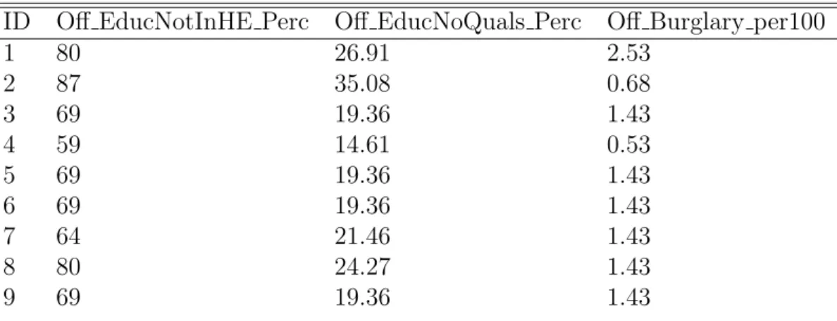
Table 2.3: WIMD Dataset Example (Joined to Offender Postcodes) ID Off EducNotInHE Perc Off EducNoQuals Perc Off Burglary per100

1 80 26.91 2.53 2 87 35.08 0.68 3 69 19.36 1.43 4 59 14.61 0.53 5 69 19.36 1.43 6 69 19.36 1.43 7 64 21.46 1.43 8 80 24.27 1.43 9 69 19.36 1.43

While making use of the first dataset could lead to valuable insights from an academic perspective, the results of this analysis (including the models produced) are unlikely to be helpful to Dyfed-Powys police if this historical data is not repre-sentative of their current dataset. Moreover, with an improvement in Dyfed-Powys data capture processes having been put into effect between 2014 and the current date, several of the issues with missing location fields are no longer present in this dataset, meaning that it is possible that many of the variables that rely on an ac-curate crime or offender location (including the WIMD variables and the distance between the offender’s location and the location of the crime) will be more likely to take a higher level of importance in the model. As such, our third dataset will be a further anonymised dataset from Dyfed-Powys police, which gives a full picture of all crimes reported to the force between 1/1/2011 and 31/12/2017. This will be known as the ”live test” data. As Dyfed-Powys have not made any additional data available for capture between the original and the ”live test” dataset, the form of this dataset will be identical to the first.

(23)

2.2.1 Dependent Variable

The Reoffence Variable Keeping in common with most previous studies (dis-counting those that defined a reoffence as a return to prison), a reoffence will be defined to be to be a further offence committed by the same offender within three years of the most recent reported offence date. Since this is a binary classification problem, the dependent variable Reoffend = 0 when an offence does not lead to a reoffence and Reoffend = 1 when an offence does lead to a reoffence. For the fol-lowing reasons, however, not all further offences reported within a three year period will be considered to be a reoffence.

What is Considered to be a Reoffence? The two variables within our dataset that will be used to define whether an offence is considered to be a reoffence are

TimeSincePrevious, defined as the number of days since the offender’s most recent offence, andNoPreviousArrests. The former variable is based on the latter, with an offence only contributing to the TimeSincePrevious variable if it adds to No-PreviousArrests. In this thesis, a ”reoffence” will correspond to a record for which the variable NoPreviousArrests ¿ 0 and the variable TimeSincePrevious ≤ 1095. Examples of this are given in Table 2.4:

Table 2.4: No. Previous Arrests: Examples

Record Offender ID TimeSincePrevious NoPreviousArrests Reoffence?

1 A 1090 1 Yes 2 B 5 0 Yes 3 B 105 1 Yes 4 B 2015 2 No 5 C 0 0 No 6 C 1250 0 No

For offender B, their 1st and 2nd offences will be counted as reoffences, but their 3rd offence will not be - this is because the 3rd offence was committed 2015 days after the 2nd one and so will be considered to be an independent offence - the No. of Previous Arrests undergone by the offender will still be accounted for, however.

To clarify, NoPreviousArrests, though not a complete misnomer, does not strictly stand for the actual number of times the offender has been arrested; this variable is an estimate, but not an actual tally, of the offender’s number of previous arrests.

(24)

Specifically, it is the number of previous crimes that the offender has committed, discounting any offences that were reported on the same date from the total. As such, an individual with two crimes reported on the same date but no previous of-fences will not be considered to have committed a reoffence with the second crime. From a policing perspective, this treatment of reoffences is much more intuitive; if an arrest is made for more than one offence, it can be very difficult or even impossi-ble to determine which of the offences is the ”original offence” and therefore, which of the offences can be considered to be ”reoffences”.

Which Offences Don’t Count Towards the Reoffence Total? To avoid con-fusion and complications with the decision as to whether or not a particular type of offence really ”counts” as a reoffence, offences that fall into the following categories will be excluded from the dataset:

1. Offences that are reported as TIC, or ”Taken Into Consideration”. These offences have been excluded due to the uncertain nature of their reporting and treatment by the justice system. The fact that these offences can be reported some time before the offender is brought to justice also complicates the calculation of how many of-fences the offender can actually be considered to have committed. While the records (dataset rows) containing TIC offences will be removed from the dataset, they will count towards the total number of arrests if they were reported at different times.

2. Offences that have not lead to any kind of prosecution by the police. This lack of prosecution can occur for many reasons, which include the decision by either the CPS or acting officer that prosecution would not be in the interest of the pub-lic, or the death or serious illness of the offender involved. Since the police do not consider these entries to be offences, they will not be considered to contribute to an offender’s offence history. These offences will be removed for prediction and will not count towards an offender’s offence history in any way.

The precise practical difference between 1 and 2 can be illustrated in the follow-ing way:

(25)

While under questioning, the offender is asked whether or not they have committed any other offences (perhaps because the police are suspicious that they may have been involved, or may have some evidence to that effect). If they do admit to fur-ther offences, the outcome of the offence may be TIC, or ”Taken Into Consideration”.

2. Suppose that the same offender is brought in for the same offence. While under questioning, the police decide that it is not worth prosecuting the offender - perhaps they decide that the reported offence is not actually an offence, or the individual who reported the offence decides not to prosecute. In this case, the outcome of the offence will be registered as ”Not A Crime” or ”Not Prosecuted”

Now that what is considered to be a reoffence has been defined, the nature of the independent variables that will be used to predict the reoffence outcome will be discussed.

2.2.2 Independent Variables

In this analysis, it was decided to investigate the maximum number of available variables for prediction. Although previous studies do give some idea of the likely most effective predictors of recidivism, including the age and sex of the offender [9] and the sanction imposed on their most recent offence [42], it is unknown if there may be other factors, of which many have not been considered by these studies, that will have a large effect an offender’s risk of recidivism.

The independent variables that have been selected and their properties, which have been extracted both from information already routinely collected by Dyfed-Powys police and the Welsh Index of Multiple Deprivation, are fully detailed in Table 1 of the Appendix. Here, some of the less obviously definable variables within this dataset will briefly be outlined.

OffenceCode

Firstly, the types of offence (OffenceCat) that individual offences are categorised by will be outlined. In the Dyfed-Powys police dataset, the offence is classified by a variable known as OffenceCode, which details the specific type of offence that

(26)

has been committed under UK law. However, since OffenceCode contains over 50 different categories, these will be re-mapped into categories based on higher-level crime classifications utilised across the UK police force. These categories are outlined in Table 2.5 below.

Table 2.5: Offence Types as Used to Categorise Crime OffenceCat Description of Offence

BurgDW Burglary Committed in a Dwelling BurgNDW Burglary Not Committed in a Dwelling CrimDam Criminal Damage

DrugPoss Drug Offence (Possession) DrugOth Drug Offence (Other) Misc Miscellaneous Offence Sex Sex Offence

Theft Theft

Violence Violent Offence

Weapon Weapon-Related Offence

Although the official guidelines sometimes separate violent offences into two dif-ferent categories depending on the level of injury caused to the victim, it has been chosen to include any offences related to violence in the same category. This is due to the fact that considering the level of harm the offence presents to society (and therefore, in this case, the severity of the injury to the person) makes the distinction between violent offences with and without injury to the person largely redundant. Since many of the public order offences also involve violence or at the very least harassment, this category has been merged into the violent offence category, with (once again) the level of harm to society done by such an offence to be determined by the variables that are generated by the crime harm values as defined by the Cambridge Crime Harm Index.

Cambridge Crime Harm Index

Level of Harm to Society Following recent research in the field [79], the Cam-bridge Crime Harm Index will be considered as a possible method of measuring the severity of an offence from the perspective of the level of harm it likely brings to society. This method, which assigns a number to a type of crime based on the likely minimum sentence or ”starting point” for that particular crime, will provide a dif-ferent perspective on crime classification grounded in the likely level of harm that

(27)

the crime presents to society. While this index does not cover all crimes recorded in this dataset as it excludes crime that is recorded due to random detection by police or security officers (i.e. drug arrests, traffic arrests, some cases of shoplifting), it is worth investigating whether or not a slightly modified version of this index would be a useful predictor of an individual’s tendency to reoffend.

The harm index with corresponding number of sentencing days attached, as it ap-pears in the original paper, is detailed in Table 2.6 below:

Table 2.6: Cambridge Crime Harm Index [79] Crime Type Subtype Starting Point Sentence Days

Homicide 5475 GBH Intent 1460 ABH 20 Assault 1 Rape 1825 Sexual Assault 365 Robbery 365 Burglary Dwelling 20 Burglary Non-Dwelling 20 Vehicle Theft of 20 Vehicle Theft from 2 Theft from Person 20 Theft from Shop 2 Theft from Other 2 Criminal Damage Arson 33 Criminal Damage Other 2

Fraud 20

These values, which are attached to each individual crime, are stored in the database as either Fine or Sentence variables depending on whether the value cor-responds to paying off a minimum fine or serving a minimum sentence.

In order to provide as full a picture as possible of the offender’s history, if a crim-inal history is present, the total past harm that the individual has inflicted upon society will also be looked into. This variable, PrevFine or PrevSentence, will be represented by the sum of the Cambridge Crime Harm Index values (stored in Fine and Sentence) of their previous crimes. This will provide a different, more specific picture to that presented by the simple number of arrests that the individual has undergone and the number of days that have passed since their previous offence.

(28)

Amendments to Cambridge Crime Harm Index To better suit the purposes of this thesis, as not all of the crimes within our dataset fit exactly into these categories, a few minor amendments to the index have been made based on CPS sentencing guidelines to cater to this particular dataset. Please note that a more detailed breakdown of the harm index for more variably charged offences such as drug possession, sexual assaults and repeat burglaries will not be in scope for this thesis, though will likely be in scope for the further development of this model as it is routinely refreshed by the police.

Table 2.7: Additions and Amendments to Cambridge Crime Harm Index Crime Type Subtype Min.Sentence Days

Kidnap 548

Death by Dangerous Driving 365

GBH Without Intent 365

Drug Offences 0

Firearms Offences 1825

Uncategorised Offences With Victim 1 Uncategorised Victimless Offences 0

Urban Rural Classification

The final variable to be introduced is a variable that quantifies the rural/urban status of a location. In this case, it has been chosen to use the classification as defined for each census output area, matching these to the postcode sectors within each area to attain a rural-urban classification for each postcode sector. This system breaks down the rural/urban classification of areas into 10 different categories, some of which are dependent on the general population density of the surrounding area. Details of exactly how these classifications were arrived at can be found on the UK Government website [25]. The 10 categories that have been used in this analysis are outlined in Table 2.8 below:

(29)

Table 2.8: Urban Rural Classification Categories, 2011 Classification Description Code

Urban Major Conurbation Not in Dataset Urban Minor Conurbation Not in Dataset

Urban City and Town 1

Urban City and Town in a Sparse Setting 2

Rural Town and Fringe 3

Rural Town and Fringe in a Sparse Setting 4

Rural Village 5

Rural Village in a Sparse Setting 6 Rural Hamlets and Isolated Dwellings 7 Rural Hamlets and Isolated Dwellings in a Sparse Setting 8

As there are no conurbations within the Dyfed-Powys policing area, it has been chosen to simply number each of the different classifications with the numbers 1-8. These will not, however, be used as an ordinal scale; these are simply categories that have been designated integer numbers for convenience.

Other Data Items

Alcohol and Drug Related Offences An interesting issue that arises for certain variables within the dataset, such whether or not an offence is Alcohol or Drug Related, is that these variables are entirely based on the immediate observations of individual officers. As such, the decision as to whether or not an offence is Alcohol or Drug Related, as well as whether or not this statistic is even recorded, may be somewhat subjective. This does not mean, however, that such information will not be useful in the analysis; it simply means that this subjectivity must be borne in mind when including this information as a predictor of reoffence.

(30)

Offence Categorisation A similar issue also arises with the categorisation of offence types and the level of harm these offences are deemed to cause on society; although the possible categories of offence types have been set as per the official UK police categorisations and the level of harm as per the Cambridge Crime Harm Index with some minor amendments, this categorisation is still somewhat subjective and there may be more useful ways of categorising these offences in a predictive situation. For the purposes of this analysis, however, the outlines provided here will be sufficient.

Dimensionality Reduction

The principle of dimensionality reduction aims to exploit the redundancy of vari-ables within input data in order to find a smaller set of new varivari-ables, which are made up of a combination of the set of the input variables fed into the technique [81]. This technique is particularly useful when attempting to fit a model to a dataset with a number of highly correlated variables.

While there are not a large number of variables to investigate in this case and it is therefore unlikely to be useful to investigate a large number of dimensionality reduction techniques for this particular dataset, there are a small number of highly correlated variables within the WIMD dataset that may benefit from the use of a dimensionality reduction technique. Moreover, making use of a smaller number of variables reduces model size, complexity and processing time, which are all concerns for Dyfed-Powys police - with limited computing power and space, reducing the size of the model will allow the police to refresh the model on a regular basis, allowing it to be kept up to date.

To illustrate the correlation between various variables in this dataset, all WIMD variables that have a correlation of at least 0.7 with another WIMD variable in the original dataset are listed in Table 2.9 below.

(31)

Table 2.9: Highly-Correlated WIMD Variables (Correlation > 0.7). See Appendix for descriptions and explanations of independent variables.

Factor Max. Correlation Max. Correlation Variable Off EmpBenefits Perc 0.9370 Off Income Perc

Crime EmpBenefits Perc 0.9395 Crime Income Perc Off Income Perc 0.9370 Off EmpBenefits Perc Crime Income Perc 0.9395 Crime EmpBenefits Perc Off EducNoQuals Perc 0.8761 Off Income Perc

Crime EmpLTSick per100000 0.8853 Crime EmpBenefits Perc Crime EducNoQuals Perc 0.8707 Crime Income Perc Off EmpLTSick per100000 0.8961 Off EmpBenefits Perc Off EducAbs Perc 0.7739 Off Income Perc Off EducNotInHE Perc 0.8296 Off Income Perc

Crime EducAbs Perc 0.7735 Crime EmpBenefits Perc Off EducKS4L2 Perc 0.8295 Off EducKS4 Pts

Crime EducKS4L2 Perc 0.7955 Crime EducKS4 Pts Off ASB per100 0.8704 Off Violence per100 Crime ASB per100 0.9140 Crime Violence per100 Off CrimDam per100 0.8750 Off Violence per100 Crime CrimDam per100 0.9326 Crime Violence per100 Crime Fire per100 0.7185 Crime ASB per100

In this case, it has been chosen to make use of one of the simplest and most widely-used dimensionality reduction techniques, Principal Components Analysis [64]. This technique was chosen for its explainability and wide use in many mathe-matical, statistical and data science contexts - this technique should be familiar to many members of staff within Dyfed-Powys police and should be simple to explain to higher-up staff members, if an explanation is requested.

PCA converts a set of observations of possibly correlated variables (in this case, a set of numerical variables relating to two potentially separate geographic areas, of which some are highly correlated) into a set of linearly uncorrelated variables known as Principal Components. These components are defined such that the first of these components accounts for as much of the variability in the data as possible. Succes-sive components will then have the highest variance possible under the constraint that they are orthogonal to all preceding components.

Defining this input set of WIMD variables to be w, the first step is to look for a linear function αT₁w of the elements of w with maximum variance. Here, αT₁ is a transposed vector of p constants α11, α12, ..., α1p, such that:

(32)

αT₁w=α11w1+α12w2+...+α1pwp = p

X

j=1

α1jwj (2.1)

In successive steps for all k > 1, a linear function αT_kw uncorrelated with

αT

1w, ..., αTk−1w that has maximum variance will be found. The kth derived

vari-able using this method, αT_kw, is the kth Principal Component [44].

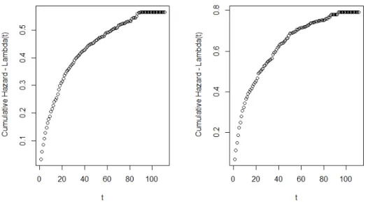
Applying Principal Components Analysis to our set of input variables w, each Prin-cipal Component generated can be plotted against the cumulative proportion of variance explained by the successive components in order to determine how many components are necessary in order to explain a sufficient proportion of the variance. This plot of the analysis conducted on the WIMD features is included in Figure 2.1 below.

Figure 2.1: Principal Components Analysis, WIMD Features

As shown above, around 30% of the total variance can be explained by the first component and around 70% by the first 5. 95% of the variance, a proportion of the variance that would be considered appropriate for these Principal Components to be used in place of the raw features, is not explained until 21 Principal Components has been reached. At this level, unless a large improvement can be made in terms of model fit or predictive ability, the loss of information and model explainability resulting from the PCA process is unlikely to outweigh the modelling benefits from

(33)

this process. As such, if this process does not offer any major benefits on the first model tested, its testing will not be extended to further models.

2.3 Algorithms for Prediction

Now that it has been discussed how the relevant algorithms will be applied in the context of this dataset, each of the algorithms to be used to predict an offender’s likelihood of recidivism will be outlined. As the focus of this thesis is to use the most recent machine learning methods to predict the occurrence of crime, it has been chosen to avoid traditional statistical methods such as Binomial Generalised Linear Models (GLMs). Binomial GLMs, in particular, have been avoided for the reason that these models (without the proper training and relevant statistical background) can be mathematically complicated and difficult to understand and maintain - this would therefore defeat the purpose of this research, which is to provide a simple, easy to deploy model to the police that can be maintained and refreshed over a period of time.

The three models that have been chosen for investigation, as previously stated in the introduction, are Random Forests, XGBoost and Neural Networks. Each of these models will now be outlined in turn, along with the advantages and disadvantages of each in a policing context, beginning with Random Forests.

2.3.1 Random Forests

The Random Forests method is a Decision Tree-based ensemble learning method not based solely on parameterised families of probability distributions[15]. It uses the technique of bootstrap aggregation to improve the unstable Decision Tree procedure [14] on many deep decision trees, producing a more stable set of classifications that have a much lower tendency to overfit to the training data than classifications pro-duced by a single decision tree. The approach exhibited by Random Forests is very suited to automatically uncovering complex data structures. In particular, the Ran-dom Forests algorithm has the ability to handle a large number of variables of both categorical and numerical types, independent variables that have non-linear effects on the dependent variable, or interactions between independent variables. In the

(34)

implementation that has been chosen, R’s Ranger [93] package, the Decision Trees will be split according to the rules of the CART algorithm and the ”best splits” found through the Gini Impurity.

Here, the method by which Random Forests are used to assess the risk of recidivism for each crime in the dataset will be outlined. This risk assessment will firstly be completed by classifying each crime as one that will lead to a reoffence or not, then producing an estimate of the probability that the crime in question will lead to a reoffence.

Random Forests for Classification

For this dataset, the Random Forests algorithm classifies variables and calculates probabilities of class membership (i.e. will or will not reoffend) in the following way:

1. For each of a series of m crimes c1,..., cm ∈ Rn, take the independent vari-ables attached to this claim to be a set of values x1, ..., xn and the corresponding reoffence indicator variable for each of these crimes to be a seriesy1, ..., ym∈R, also of length m.

2. Select a number of Decision Trees, b, to be grown for the forest.

3. For each of the b Decision Trees, sample, with replacement, a subset of crimes

c1, ..., ci, i < mfor each of the m crimes within the dataset. The m−i samples not included in the bootstrapping process are known as the Out Of Bag (OOB) samples in the dataset. These samples, essentially, will be used as a validation set.

4. We then randomly sample, with replacement, a subset x1, ..., xj, j < n of the

n explanatory variables within the dataset. In this case, j will be initially set to its default value,√n rounded to the next largest integer. This is the value that is most recommended for a classification task and the parameter value will be optimised using the Grid Search method.

(35)

into two separate child nodes, we consider all splits involving thej available features in the bootstrap sample for that tree. A new sample of j features is chosen at each node and from all splits considered using thej available features, the locally optimal split at each node is chosen based on their Gini Impurity.

6. Grow each of the b Decision Trees to their maximum depth, i.e. keep split-ting the data until it is certain that a pathway will lead to a particular outcome, or to a depth determined by a minimum node size parameter o.

7. For each of the m crimes within the dataset, take the majority vote on the classification of each crime cm as the decision as to whether or not the crime will lead to a reoffence within three years of the crime being reported.

Random Forests for Probability Estimation

If the aim is to output a probability of reoffence rather than simply classify whether or not a reoffence will occur, Step 7 can be replaced with these two steps:

7. As described in Malley et.al [55], in each of the terminal nodes of the tree, the percentage of crimes that lead to a reoffence in each terminal node is determined.

8. To estimate the probability that a given crime within themcrimes in the training set will lead to a reoffence, the crime is dropped down each of the b trees until it reaches the terminal node. The probability of reoffence (percentage of crimes that lead to a reoffence) at the crime’s terminal node is then averaged across all of theb

trees.

Use and Implications

As Random Forests can be described by taking the concept of decision trees and combining it with a concept that can essentially be described by ”taking a ma-jority vote”, this algorithm is relatively simple to understand for those with a non-mathematical background. It is also simple to add and remove factors, though these factors will require some processing, particularly if they are categorical in nature.

(36)

In terms of parameter tuning and cross-validation, beyond finding the appropriate number of trees (for which there exists a large range of ”good enough” numbers), very little tuning is necessary in order for this model to operate, as this tuning will rarely increase the predictive accuracy of the model by more than 1-2%. Nonethe-less, in order to ensure good performance, grid search was used to find the optimum value of mtry, or the number of features (j in the above description) competing at each node. While it is also possible to tune other parameters, developing new features will generally be far more effective in increasing the accuracy of the model on unseen data than altering the parameters.

Maintaining and refreshing the model is a relatively simple process, though will require some expertise to refresh it if the factors that affect reoffending change over time - though it is not expected for this to happen in the immediate future, this is always an inherent danger in modelling using historical data.

2.3.2 XGBoost

XGBoost, or extreme gradient boosting, is a scalable machine learning system for tree boosting. Among the 29 challenge winning solutions published at Kaggle’s blog during 2015, 17 of those solutions incorporated the XGBoost algorithm. In the 2015 KDDCup, an annual data mining competition, it was also used by every team in the top 10 [18]. This method, as such, is certainly worth investigating both as a viable alternative to the Random Forests algorithm and as a further investigation into the use of Gradient Boosting methods for the purposes of predicting recidivism. In general, Gradient Boosting shares some similarities with Random Forests as it can also be thought of as the process of combining multiple weak learners into a single strong learner using Gradient Descent and Boosting techniques. The weak learners in the XGBoost algorithm, like Random Forests, are CART trees. However, unlike Random Forests, the trees are grown to a fixed size and are not allowed to reach their maximum possible depth.

As before, the aim of this algorithm is to teach a model (in this case, a number of CART trees) to predict whether or not an offence will lead to a reoffence within three years, as indicated by reoffence indicator variables y = y1, ..., ym ∈ R, for a

(37)

test set of m crimes c1, c2, ..., cm ∈ Rn with corresponding independent variables

x = x1, ..., xn. Rather than simply setting a number of trees, the learning in XG-Boost is completed over a series of iterations 1≤ b≤ B, where B is the maximum number of iterations set by the user. For a number of CART trees B (keeping the notation consistent with Random Forests), the prediction generated by the model for the reoffence outcome of an individual crime ˆyi is generated as follows:

1. An initial model F1(x) is fitted to the set of reoffence indicators, y. In this

case, this will be a Decision Tree that attempts to predict an offender’s probability of reoffence.

2. The residuals of this model, y −F1(x) are then taken and a model, f1(x), is

fit to the residuals. By fitting a further decision tree to just the cases where our model produced incorrect predictions, the aim is to find a pattern within this seg-ment of the data that our initial model may have missed.

3. This model, f1(x), is then added to the first model to make a new model F2(x),

as follows:

F2(x) =F1(x) +f1(x) (2.2)

This process of taking a previous model, finding the residuals, fitting a model (Decision Tree) to these residuals and adding this to the previous model then con-tinues until either:

1. A Loss Function is minimised as follows:

L=X i l(ˆyi, yi) + X b Ω(Fb) (2.3)

The first term, l(ˆyi, yi), is a differentiable convex loss function measuring the difference between the predicted value ˆyi and the target value yi. In the XGBoost package for R [19], several different evaluation metrics are available. The second term Ω(F), where Ω(F) =γE+1₂λ||w||2 _{is a term that penalises the complexity of}

each of the CART trees (in this case, E represents the number of leaves in the tree and w the weights applied to those leaves). When this regularisation term is set to

(38)

0, traditional gradient tree boosting is used.

2. Reach a point where the the process has been told to stop. The most com-mon way of doing this is by using an early stopping procedure, which will evaluate the progress of the objective function’s minimisation and bring learning to a stop when the objective function is no longer significantly improving (the aforementioned ”significance” being set by a given level of tolerance).

In either case, a model comprising a number of Decision Trees, B, will eventually be arrived at as follows: ˆ y=FB(x) = F1(x) +η( B−1 X b=1 fb(x)) (2.4)

In this equation,η is the learning rate of the function, which controls the weight-ing of new trees that are added to the model. This is an important parameter that must be tuned in order to avoid overfitting and as before, we made use of grid search to tune this parameter within reasonable bounds. To minimise an objective, tra-ditional optimisation methods in Euclidean space cannot be used, due to the fact that functions are included as parameters. This is the reason why the model must be trained in an additive manner over a number of iterations 1< b≤B rather than in a single step.

Objectives are optimised at each iteration b, the first and second order gradient statistics on the loss function are introduced so that a second order approximation can be used to quickly optimise this objective. Similarly to the Gini Impurity score that is usually used to evaluate decision trees, XGBoost uses this function as a scor-ing function to measure the quality of an individual tree structure b.

As it is usually impossible to enumerate all possible tree structures b, however, a greedy algorithm (i.e. one that follows the heuristic of making locally optimal choices in order to find a global optimum) that begins from a single leaf E and iteratively adds branches to each tree b is used instead. To find this best split and to decide which values of which features should be considered for splitting, an ap-proximate version of the exact greedy algorithm, i.e. an algorithm that enumerates

(39)

over all possible splits on all features in order to find the best split, is used. This algorithm, instead of looking at all possible values of features, proposes split points according to percentiles of feature distribution. The XGBoost implementation of gradient boosting is also sparsity-aware, making it suitable for use with sparse input data.

Use and Implications

Once again, the XGBoost algorithm is based on decision trees, which makes it rel-atively simple to explain to those of a non-mathematical background. However, as the process requires the iterative addition of further trees that are fit on to the resid-uals of the first tree, it can be more difficult to visualise how this algorithm works than it will be for Random Forests. In the same vein as Random Forests, however, it is also simple to add and remove factors, though these factors will require some processing, particularly if they are categorical in nature.

In terms of parameter tuning and cross-validation, due to the nature of the XG-Boost algorithm, slightly more care must be taken in order to avoid overfitting the model to the training data, particularly in terms of finding the optimal number of steps to maximise the fit to unseen data. Moreover, the parameters that control the gradient descent (in particular, the learning rate of the algorithm), will require adjustment every time. This will require some understanding of the process of gra-dient descent on the part of the police, which may or may not already be within their base of specific knowledge.

Maintaining and refreshing the model is, therefore a slightly more complex pro-cess compared to the propro-cess of maintaining and refreshing Random Forests. Once an appropriate cross-validation process is set up and understood, however, the only real issue appears in (as previously discussed) dealing with the possibility that the factors affecting reoffending will change over time.

2.3.3 Neural Networks

Artificial Neural Networks are computing systems inspired by biological neural net-works within animal brains. These netnet-works consist of a set of artificial neurons

(40)

(nodes) that produce a series of real-valued activations, joined by a series of directed edges, representing the synapses connecting these neurons. They are designed to in-terpret sensory data as received by input neurons, which must be numerical and in vector form, in order to recognise and exploit patterns within a given dataset. In these networks, input neurons are activated by sensors that perceive the en-vironment, while other neurons are activated through weighted connections from previously activated neurons. Networks learn or assign credit by iteratively updat-ing the aforementioned weights until the network exhibits the desired behaviour; in our case, this will be producing an accurate prediction as to whether or not a crime will lead to a reoffence within 3 years of its reported date.

In general, Neural Networks can be used to solve many different types of problems. For standard supervised learning classification tasks like this one, which require hu-man knowledge of a dataset in order for a neural network to learn the correlation between a dataset and the labels attached to each observation, many different types of Neural Networks can be used. A series of Feedforward (acyclic) Neural Networks will therefore be built to make use of the independent variables in our dataset to determine whether or not an individual crime will lead to a reoffence within 3 years of the reported date. PCA analysis will not be incorporated into this section.

Neural Network Architectures

The layers in a neural network are made of a finite number H of interconnected nodes, h, which are associated with an activation function ah(·). Each edge in the finite set of edgesD that connects a node hto another node h0 is associated with a weight w_hh0, which assigns a level of importance to the value of the input from the

previous node. The valuevhoutput by each nodehis then calculated by applying the activation function ah to a weighted sum of the values of its input nodes, according to the weights w_hh0. vh =ah X h0 w_hh0 ·v h0 (2.5)

The Neural Network architecture of a Feedforward Neural Network with Llayers is constructed as follows: