This is the author’s version of a work that was submitted/accepted for pub-lication in the following source:
Nantes, Alfredo,Miska, Marc Philipp,Bhaskar, Ashish, &Chung, Edward (2014) Noisy Bluetooth traffic data? ARRB Road & Transport Research
Journal,23(1), pp. 33-43.
This file was downloaded from: http://eprints.qut.edu.au/72697/
c
Copyright 2014 A R R B Group Ltd
Notice: Changes introduced as a result of publishing processes such as
copy-editing and formatting may not be reflected in this document. For a definitive version of this work, please refer to the published source:
Noisy Bluetooth Traffic Data?
Dr. Alfredo Nantes (
corresponding author
)
Smart Transport Research Centre,
Science and Engineering Faculty,
Queensland University of Technology
2 George St GPO Box 2434, Brisbane QLD 4001 – Australia
Tel: +61 7 3138 1461
Email: [email protected]
Dr. Marc Philipp Miska
Smart Transport Research Centre,
Science and Engineering Faculty,
Queensland University of Technology
2 George St GPO Box 2434, Brisbane QLD 4001 – Australia
Dr. Ashish Bhaskar
Smart Transport Research Centre,
Science and Engineering Faculty,
Queensland University of Technology
2 George St GPO Box 2434, Brisbane QLD 4001 – Australia
Prof. Dr. Edward Chung
Smart Transport Research Centre,
Science and Engineering Faculty,
Queensland University of Technology
2 George St GPO Box 2434, Brisbane QLD 4001 - Australia
Abstract
Traffic state estimation in an urban road network remains a challenge for traffic models and the question of how such a network performs remains a difficult one to answer for traffic operators. Lack of detailed traffic information has long restricted research in this area. The introduction of Bluetooth into the automotive world presented an alternative that has now developed to a stage where large-‐scale test-‐beds are becoming available, for traffic monitoring and model validation purposes. But how much confidence should we have in such data?
This paper aims to give an overview of the usage of Bluetooth, primarily for the city-‐scale management of urban transport networks, and to encourage researchers and practitioners to take a more cautious look at what is currently understood as a mature technology for monitoring travellers in urban environments. We argue that the full value of this technology is yet to be realized, for the analytical accuracies peculiar to the data have still to be adequately resolved.
Introduction
Traffic is a complex, non-‐linear and non-‐stationary process that exhibits different levels of organization; ranging from the driver-‐vehicle interaction [1], to the microscopic behaviour of individual drivers [2], to the macroscopic behaviour of road stretches and networks [3-‐7]. Understanding the traffic dynamics has proven very challenging, especially in the presence of hindrances peculiar to urban road networks, such as pedestrian crossings, traffic signals and intersections. The lack of traffic data has traditionally prevented researchers from gaining detailed insight into the mechanistic basis of the traffic processes. In recent years however, technological advances have been made in the area of road and in-‐vehicle telematics, which have led to the collection of large amounts of new road data. This new data has, in turn, given new vigour to theoretical work in the area of Intelligent Transport Systems (ITS).
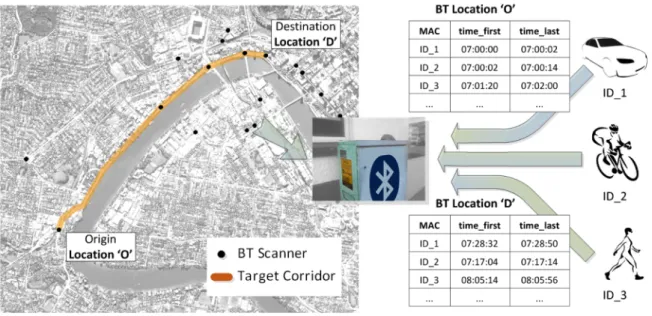
The current state of the practice among researchers and in various departments of transportation is to collect Bluetooth data, and use this in combination with other sources in order to sample important traffic parameters, such as speed, flow and density [8-‐11]. The Bluetooth scanners sample the road traffic by capturing the electronic identifiers, or MAC addresses, of the Bluetooth-‐enabled devices that transits within the scanning area. Along with the MAC addresses, the times at which the devices are first and last detected are recorded (Figure 1). Because the MAC addresses are unique and all scanners are time-‐synchronized, the activity of the individual road users can be monitored. Over the past decade, there has been a relatively comprehensive experience with the Bluetooth technology in transport and other sectors, across the world. Considerable research has been conducted on the estimation of the experienced travel times and the root choice of the users [12-‐ 17]. Recently, researchers have also attempted to reconstruct the full state of traffic from the partial, noisy Bluetooth observations [9, 17]. Very few attempts, however, have been made towards understanding the source of noise and the accuracies peculiar to the data. At best, the Bluetooth noise is assumed to have a (simple) known distribution, with parameters that are not derived from the characteristics of the scanners, or from any other evidence. Needless to say, improper scanner models yield estimations that may diverge considerably from the actual traffic situation, now matter how accurate the underpinning traffic models are.
In the next sections, we will give an overview of the history of Bluetooth technology applied to transport and other sectors. Two main sections will then follow, in which we will discuss the noise components of the Bluetooth data and will bring a new outlook to the way the data is pre-‐processed and analysed, in order to address two related transport problems: the estimation of travel times and route choices. Conclusions will be drawn in the final section.
The Birth of the Bluetooth Traffic Data Sensing
The usage of Bluetooth in transport has passed its first decade, and though it has come a long way, its full potential is still to be explored. In the early days, [18] investigated the utilization of Bluetooth for short-‐term ad hoc connections between moving vehicles, while it was still a new wireless technology. The findings were promising. They showed that even fast vehicles -‐ driving 100 km/h – could be detected by a Class 1 (20dB) Bluetooth. Although the experiments were performed for vehicle-‐to-‐vehicle communication, the same issues apply to monitoring traffic through Bluetooth scanners. In the same year, Sergio Luciani, submitted an application to the United States Patent office that described, though as a fall back option, exactly that: The usage of Bluetooth scanners for traffic monitoring. In his application, Luciani [19] described that tracking the MAC address of a device along the road through matching sighting with paths through the road network, one would be able to determine travel times that, when compared to a baseline, could be used to determine the traffic state of the road. The patent was issued one year later in 2003. While the described setup is similar to what is used today, it took years to see it established on the road. Though the idea of using Bluetooth, among other mobile sensors, for traffic monitoring manifested itself in various sensor network based traffic information service systems (SNTISS), such as the three-‐tiered architecture proposed by [20]. By that time it was clear that intelligent transport systems (ITS) would require networks of smart sensors embedded in the traffic area, performing automated continual and pervasive monitoring to enhance the quality of traffic information collection and services.
It took another three years before [21] introduced a prototypical implementation and test deployment of a Bluetooth and wireless mesh networks platform for traffic network monitoring. The platform used cars as mobile sensors and used wireless municipal mesh networks to transport the sensed data. The assumption was that drivers carry mobile devices equipped with the widely adopted low-‐cost Bluetooth wireless technology. The platform was able to track cars travelling at speeds of 0 to 70 km/hour. In addition to tracking vehicles, the study was able to approximate car
Figure 1: Bluetooth probing strategy. Bluetooth scanners probe road networks by recording MAC addresses of the detected devices, and times of first and last detection. These data enable to monitor the users’ activity (e.g. travel time and demand) for the target corridors.
speeds with an accuracy of ± 15%. A similar study was performed by Mohan, et al. [22] who suggested the system as a cost effective solution for developing countries. One year later, and with large sample sizes of 5% to 7% of the overall traffic stream, Tarnoff et al. [23] introduced a system claiming accurate measurement of travel times as well as origin-‐destination data for freeway and arterial roadway networks. The paper points out that the major benefits are that the cost of Bluetooth scanning are a factor of 100 less than equivalent floating car runs, and that privacy is less of an issue with the Bluetooth equipment due to the absence of databases that can relate addresses to specific individuals (owners). Another system was developed to ease the path for road authorities to enter the travel time measurement market by Puckett and Vickich [24], who took a practitioners’ approach. The accuracy of travel time measurement, and the ease on the privacy issue, that made the usage of mobile phone data nearly impossible, might have been the turning point, as from then on Bluetooth gained a lot more interest from the research community.
Experiences and Case Studies
Over the past few years, the Bluetooth data source has been used for large-‐scale behavior studies, across different domains. It has been used to characterize pedestrian environments and walking behavior, by using the distributions of device type, dwell time and travel time [25, 26]. These endeavors have been directed towards the analysis of the effect of the environment on the signal strength of the scanners, and the relationship between the signal strength and type and frequency of detection road users such as walkers, runners and cyclists [27]. Recently, researchers have used the Bluetooth-‐based tracking strategy to measure the time it takes for passengers to move through the various airport areas [28]. Currently, Bluetooth finds its widest application within the Intelligent Transport System and Road Management domains. Here, the Bluetooth data are often fused with other data sources -‐ such as WiFi, GPS and loop detectors [29] -‐ in order to enhance the estimation of the traffic state or to identify the causes of congestion outbreaks [9]. Finally, the Bluetooth technologyhas also been recently employed for improving the estimation of Origin-‐Destination patterns [30] and route choice analysis [31, 32].
The Bluetooth-‐Based Estimation of Travel Time
The Travel Time is an important traffic indicator of the status of the network and may be used to minimize the level of congestion. It has long been a topic of research and numerous models have been proposed for both motorways [33-‐42] and arterial [43-‐46] networks. The relationship between the level of congestion and travel time has been studied theoretically by a number of researchers [4, 47] and has led to the conclusion that, if the vast majority of drivers were informed on the actual travel time for their trips, congestion would be reduced significantly, provided that these drivers made the right decision at the right time, in a cooperative fashion [48].
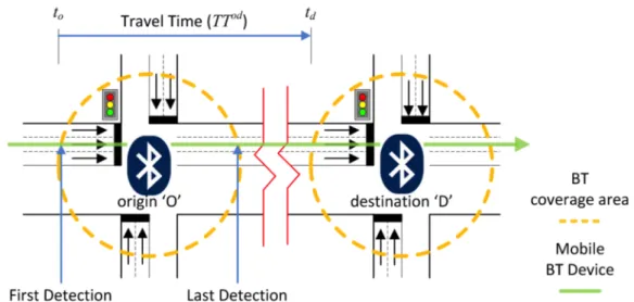
It is one thing, however, to assume that the output from a traffic simulator is realistic, and quite another thing trying to determine how realistic this output is, when the parameters of the simulator are numerous and the data available for validation are very limited and noisy. A very important validation data seemed to become available at a low cost when it was shown by Murphy et al. [18] that pairing Bluetooth sensors together could produce travel time data. Simply put, given a pair of locations, 𝑂 and 𝐷, both covered by Bluetooth scanners, the time it takes for a Bluetooth discoverable traveller to go from 𝑂 to 𝐷 is given by the time difference between the matching identifiers (Figure 2). Therefore, if a vehicle is first detected at 𝑂 at time 𝑡!, and later at 𝐷 at time 𝑡!,
the travel time 𝜏(𝑂,𝐷) for this device will simply be
𝜏(𝑂,𝐷)=𝑡!−𝑡!
(1)
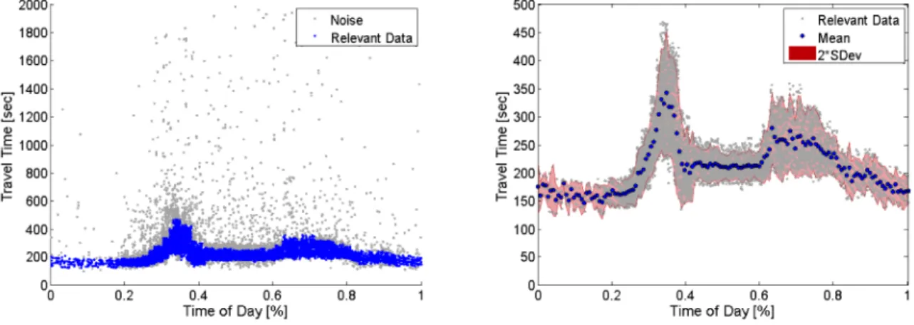
By plotting these values over some period of time (Figure 3, left), the travel time stands out, from what is seems like feeble background noise. Since the early promising reports on the use of the Bluetooth technology for traffic monitoring, researchers and practitioners have been debating about the actual value of this relatively new data source. Strictly speaking, although the mechanisms for measuring the travel time seems simple and does produce large datasets, it is still not clear how much noise is actually ‘lurking’ in the data and how this noise ought to be isolated and reduced.
Figure 3: Travel Time de-‐noising and parameterization. Common travel time measures for a corridor are produced from the aggregation of per-‐vehicle travel times over a given time window, e.g. 1 day (left). Data cleansing is often achieved by separating high-‐density regions from the regions of low density. From the cleansed data (dark-‐blue region on the left picture), sufficient statistics (e.g. mean and standard deviation) are computed and used as indicators of road performance (right). The filtered data in this example was clustered into 144 time bins of equal length. Mean and standard deviation were then computed for each time bin. In the graph on the left, the red region indicates the
Travel Time Modes and Noise
What both researchers and practitioners know is that the Bluetooth data typically hides the traffic mode of the detected travellers. Within any Bluetooth dataset, one should expect to find samples belonging to the class of personal cars, pedestrians, busses, taxies, cyclists and all kinds of road users. Not all these data points are equally important as far as vehicular traffic is concerned. Yet, they do equally influence the sufficient statistics that are to be computed, as a summary of the large dataset, if the priors of each mode are not known. This difficulty is typically addressed as follows. If one assumed that the outliers, e.g. the non-‐target transport modes, were more scattered or less dense in the dataset, and the samples of the target class closer together, then clustering techniques could be used to identify and filter the target class from the rest of the dataset. This modus-‐operandi branches out into two major strategies. One strategy, which we shall term static, consists of slicing time into bins within which the (travel time) data is partitioned. Then for each bin, a second clustering is applied in order to discern between dense (target) versus scattered (non-‐target) regions [17, 49, 50]. An example of this approach is depicted in the right diagram of Figure 3. The second approach is more dynamic, in the sense that the output of the clustering algorithm depends also on the data from the previous time-‐steps. If different transport modes exhibit different density patterns in the data, the dynamic approach is expected to enable more robust filtering and even prediction [8, 51].
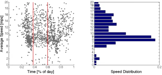
But do we always see these patterns of high and low-‐density regions in the travel time data? And are the high-‐density regions actually characteristic of the target class? Under certain circumstances, both questions may have a positive answer. Let us assume that we were to target the class of motorized vehicles. Intuitively, motorized vehicles tend to be faster than pedestrian and cyclists, provided that the traffic were not congested. Therefore, we would expect to see at least two modes in the travel time (average speed) distribution: a higher travel time (lower average speed) peak for the non-‐motorized vehicles and a lower travel time (higher average speed) peak caused by the
Figure 4: Average speed measured between two scanned intersections. The speed distribution for the target corridor (Coronation Drive, Brisbane) appears to be multi-‐modal between 9am (~40% of one day) and 3pm (~60% of one day).
motorized vehicles. In this situation, any classifier is expected to place a decision boundary somewhere between these two classes. As congestion kicks in, these two classes will gradually come closer together and merge, at the point in time when the average speed of cars and pedestrians would no longer be statistically distinguishable.
What about the density patterns? Until recently, it seemed safe to consider the data coming from mobile phones and smartphones less abundant, compared to the sightings from the Bluetooth-‐ enabled vehicles. Put it simply, a native support of a more powerful Bluetooth class, for a mobile device, would entail a shorter battery lifetime. However, a lower power-‐class would also translate to smaller communications ranges. By contrast, the batteries of vehicles have had the advantage of being constantly recharged by the vehicles’ engine. Therefore, there would be virtually no disadvantage in using a more powerful Bluetooth hands-‐free vehicle kit, in order to offer wider scanning ranges. Under these hypotheses, it was reasonable to conclude that the motorized versus non-‐motorized classes are characterized by different densities, in time and space. However, the new Bluetooth low energy (LE) protocol, which is being supported by an ever-‐increasing number of portable electronic devices [52], has proved successful in keeping the energy consumption to a minimum, while increasing the range to over 100 meters [53]. As the non-‐vehicular traffic becomes easier to observe, the assumption of clearly distinguishable density regions may no longer hold. In general, as the Bluetooth technology keeps improving, the assumptions made about the Bluetooth data will need to be revisited. But even if all transport classes could be perfectly separated, each class would still exhibit some degree of variance around its mean value (Figure 3, right). Part of this variance can be explained as follows. The behaviour of the individual drivers is influenced, among other things, by a number of external factors, such as traffic lights, merging and diverging flows. These factors may cause the trajectory of two nearby vehicles to diverge significantly, even over a small time window. At the one end of the spectrum we shall find the travellers experiencing the shortest travel times, as their drive will not be interrupted by any red signal or merging vehicle. At the opposite end of the spectrum, the least lucky drivers will experience the largest travel times, for being interrupted by all traffic hindrances in their way. It the case of short road links between two Bluetooth scanners, the travel time (or average speed) distribution tends to be bi-‐modal (Figure 4). In this situation no driver is likely to experience the average travel time, located somewhere between the two peaks.
The rest of the variance of the clustered and cleansed data comes from the characteristic of the sensors and can be explained more formally. The Bluetooth scanning is not continuous but it rather happens at fixed time intervals called inquiry cycles [54]. When an inquiry cycle is completed, the MAC IDs of the detected devices are sent to the main server to be time-‐stamped with the time at which the inquiry cycle call has returned. Let 𝑇! be the duration of the inquiry cycle, which we will
assume to be constant1; and 𝑇
! the duration of the data processing operations, i.e. data transfer
from scanner to server and time-‐stamping (Figure 5, left). If 𝑇! is uniformly distributed within some arbitrary interval [𝑎,𝑏] with 𝑎 and 𝑏 being non-‐negative real numbers, the measurement error 𝜉 will be distributed as depicted in Figure 5 (right). This error is the difference between the time reported or measured by the Bluetooth scanning system and the actual time at which the devices enter the scanning area. Interested readers should refer to [55] for detailed analysis on the Bluetooth data acquisition process and analysis on the noise from the data. The width of such a distribution is
postulated to be proportional to the variance that is observed around each mode of the speed or travel time distribution (Figure 4 right). In reality, this probability density function is also affected by the miss-‐detection rate, that is, the chance of a scanner to miss a discoverable device that is transiting within the scanning area. It can be shown that the higher this probability is, the wider the error distribution will become. The miss-‐detection rate depends on the dwell-‐time of a vehicle within the scanning area, and other external disturbances. For instance, the polarization of a scanner antenna (e.g. omnidirectional versus directional) defines its communication coverage shape (horizontal and vertical), and the gain (strength in dBi units) of the antenna defines the size of the coverage shape. The actual scanning shape in the real environment, in turn, is affected by the local installation factors such as attenuations and reflections to the signals from trees, buildings and even weather conditions (water absorbs radio waves at the frequencies used by Bluetooth). Low scanning frequencies and small covering areas result in a smaller chance for the fast vehicles to be timed accurately. In the worst case, vehicles are missed altogether if their transit in and out of the scanning area is very short. If we neglected the miss-‐detection chance and still wished to formulate travel time in probabilistic terms, we should modify Eq. (1) as follows:
Ε 𝜏 𝑂,𝐷 =Ε[𝑡!]+Ε[ξ]−(Ε[𝑡!]+Ε ξ)
(2)
Where Ε[∙] is the expected travel time and 𝑡! and 𝑡! are now random variables denoting the entrance time, over some period of time, at the origin and destination scanner, respectively. The equation above holds true, no matter what the distribution of ξ may be, as long as we assume that ξ is the same for all scanners. Therefore we can see that, on ‘average’, the measurement errors will cancel each other out, leaving us with the conclusion thatΕ 𝜏 𝑂,𝐷 =Ε[𝑡!−𝑡!]
(3)
which says that the mean of the measured travel time is equal to the mean of the actual travel time, regardless of the error ξ. This result may lead researchers and practitioners to ignore the nature of the Bluetooth noise, for travel time estimation purposes, and replace the random variables t! and
t! with their sufficient statistics, such as the mean. The problem with Eq. (3) is however numerical rather than theoretical. The mean computed from the (Bluetooth) data is equal to the analytical
Figure 5: Bluetooth inquiry cycles and measurement error distribution. The graph on the right shows that the measurement error depends on the time at which the individual devices enter the scanning area (entrance time) and the time at which the current inquiry process completes. This includes the random variable 𝑇!, which is assumed to be distributed uniformly between 𝑎 and 𝑏. The probability distribution of the error 𝑓(𝜉) resulting from this system is shown on the right.
mean only if the dataset, over the time period considered, were infinitely large. In practice, however, the difference between measured and analytical mean will fall within small intervals, if the sample size were big enough. By contrast, if the data were very limited over the target time window, the travel time measured could diverge significantly from the actual travel time. Thus, we have seen that not only does the Bluetooth noise have a non-‐Gaussian distribution, as is often assumes; but this noise should not be neglected, even for the simple task of estimating the travel time between to Bluetooth scanners.
Route Choice Analysis
Route choice problems in transportation modelling have been drawing the attention of researchers from different domains, including statistics [56], economics [57], AI [58] and psychology [59]. Amongst these endeavours, extensive effort has been invested to understand the mechanisms whereby people plan routes, given the objective and reward of the trip and the information that is assumed to be available to them, such as travel times, road closures and bottlenecks and traffic incidents. We are interested in route choice because of its importance in determining traffic demand. Congestion occurs when the demand for travel exceeds the capacity of the road. Therefore, analysing how and why demand changes is important to reduce congestion and, ultimately, economic and environmental damage. Moreover, understanding people choice can assist with deciding on the public transport infrastructures to build, in order to enhance the quality of life in the cities [60]. Over the years, a number of robust and efficient models have been proposed to address traffic choice problems. Despite the mathematical elegance and practical appeal of these models, their validation with real data has remained a challenge. Travel surveys and traffic simulators, have long been the methods of choice for training and validating the models [61]. However, it is commonly agreed that survey data may be strongly biased [62], as they usually involve small, randomly selected samples of the population, which may not reflect the actual overall behaviour. Moreover, the reliability of surveys depends on several factors, such as subject motivation, structure of the survey and question design. In contrast, traffic simulators produce rich, high-‐precision data, but this synthetic data may not reflect what people actually do under atypical circumstances. Similarly to the travel time estimation problem, researchers have recently explored the opportunity offered by the large datasets of Bluetooth data [63].
Travel Time-‐Based Choices
The route-‐choice problem, posed in probabilistic terms [64], requires the calculation of the conditional distribution Ψ!!", representing the driver choice of selecting a route 𝑖, from origin 𝑜 to destination 𝑑, from a set of relevant route choice set 𝐶!" . Formally, this is expressed as
Ψ!!" =Pr 𝑖 𝐶!"
(4)
Different mathematical models can be used to define the above probability, such as the Paired Combination Logit Model [65] and the Cross-‐Nested Logit Model [66]. Of all the factors impacting on the route choice of drivers, travel time is increasingly being recognized as one of the most influential [58]. If we marginalize Eq. 4 over the set of all travel times available about the routes in 𝐶!", we get:Ψ!!" =Pr 𝑖 𝐶!" = Pr 𝑖 𝜏,𝐶!" Pr 𝜏 𝐶!"
Here, it is assumed that the user choice depends on the time it takes to travel 𝐶!". This dependency is expressed by the model Pr 𝑖 𝜏,𝐶!" , that is, the probability of selecting corridor 𝑖, given 𝐶!" and the prior Pr 𝜏 𝐶!" , denoting the probability of experiencing the travel times 𝜏 when travelling 𝐶!". This latter distribution can be extracted directly from the (Bluetooth) travel time data.
One of the major issues with the estimation of the travelled path is that the Bluetooth scanners may not be located at every intersection of the target corridor. Moreover, as explained earlier, there is a chance that a scanner will not detect all vehicles that are flowing through the scanned intersection. As such, the entire trip of the road users may translate to small Bluetooth samples. Reconstructing long trips from such limited datasets may be a daunting challenge. Michau et al. [67] have recently presented a technique that allows determining a lower bound for the number of miss-‐detections and to infer about the actual travelled path. The inference is based on the statistics computed from the dataset and on a set of assumptions made about the distribution of speed across vehicles and non-‐vehicles. Their work is an attempt to include the Bluetooth-‐related uncertainties into the reconstruction of the actual path.
A second complication concerns the identification of the actual number of trips, from the series of unlabelled Bluetooth sightings. Typically, a Bluetooth dataset is made of series of per-‐traveller recordings, which refers to the times at which the traveller has ‘hit’ the various scanners, over the observation period. This series may contain multiple recordings from the same scanner and is usually unlabelled, in that, it does not contain information about the origin and destination of each trip. To address this problem it is common to resort to heuristics, which allow for the overall behaviour of the entire population of drivers. In a recent work, Michau et al. [67] have proposed speed-‐based splitting criteria, in which a split point is introduced whenever the speed between adjacent detections goes below a threshold. This method allows also for the probability of the time-‐difference between pairs of consecutive detections. In general, the splitting problem is addressed through threshold-‐based heuristics, whereby groups of trips are formed, on the basis of the frequency of consecutive recordings, among other parameters [68]. The time thresholds used, however, is not based on the characteristic behaviour of the scanners. It has been shown that the weather has a strong influence on the signal strength; that the miss-‐detection rate increases as the scanning area becomes more crowded with active Bluetooth devices and that not all scanners may be equally powerful [63]. Determining the actual origin, destination and path of the individual drivers from unlabelled Bluetooth is critical to the accuracy of any route choice model used. Yet, there has been very little contribution to incorporate these factors into a trip-‐splitting strategy. Instead, the sequences of Bluetooth observations are often associated to the shortest path connecting the hit scanners along the way, and the travel times associated with them are given through sufficient statistics.
Concluding Remarks
Technological advances in the field of vehicle telematics are having positive impact on the state-‐of-‐ the-‐art of traffic models, as they have enable the measurement of important factors such as travel time, traffic demand and route choices. In this work, we have presented examples of the application of the Bluetooth technology to behavioural studies with focus on travel time estimation and route choices modelling. We argue that for the effective estimation of any traffic-‐related information, it is important to understand and model characteristics behaviour of the Bluetooth scanners. Not only
will the understanding of the source of Bluetooth noise improve the estimation mechanisms that are currently used; but it will also help devising informed strategies for the optimal positioning and distribution of the scanners, for road and even retail management purposes. It is expected that the growth of the Bluetooth data deluge will spur more rigorous investigations along this direction. The Smart Transport Research Centre2 is already in an excellent position in this respect, as it has access
to a large Bluetooth dataset from Brisbane, with over 400 scanners. The size of this set is expected to increase considerably in the near future, and will include data from urban and sub-‐urban areas. We postulate that from such a large sample it will become easier to identify and characterize the noise that is currently hidden in the data.
References
[1] M. P. Miska, A. Nantes, B. Lee, and E. Chung, "Physically sound vehicle-‐driver model for realistic microscopic simulation," in Transportation Research Board 91st Annual Meeting 2012, Washington DC, 2012.
[2] J. Barceló and J. Casas, "Stochastic Heuristic Dynamic Assignment Based on AIMSUN Microscopic Traffic Simulator," Transportation Research Record: Journal of the Transportation Research Board, pp. 70-‐80, 2006.
[3] C. F. Daganzo, V. V. Gayah, and E. J. Gonzales, "Macroscopic relations of urban traffic variables: Bifurcations, multivaluedness and instability," Transportation Research Part B: Methodological, vol. 45, pp. 278 -‐ 288, 2011.
[4] T. Tsubota, A. Bhaskar, E. Chung, and G. Nikolas, "Information provision and network performance represented by Macroscopic Fundamental Diagram," presented at the Transportation Research Board 92nd Annual Meeting, Washington DC, USA, 2013. [5] T. Tsubota, A. Bhaskar, and E. Chung, "Empirical Evaluation of Brisbane Macroscopic
Fundamental Diagram," in 36th Australasian Transport Research Forum (ATRF), Brisbane, Australia, 2013.
[6] T. Tsubota, A. Bhaskar, E. Chung, and G. Nikolas, "Real time information provision benefit measured by macroscopic fundamental diagram," presented at the 13 World Conference on Transport Research, Rio de Janeiro, Brazil, 2013.
[7] T. Tsubota, A. Bhaskar, and C. Edward, "Brisbane Macroscopic Fundamental Diagram: Emperical Findings on Network Partitioning and Incident Detection," in Transportation Research Board 93nd Annual Meeting, Washington DC, 2014.
[8] A. Nantes, R. Billot, M. P. Miska, and E. Chung, "Bayesian Inference of Traffic Volumes Based on Bluetooth Data," presented at the Transportation Research Board 92nd Annual Meeting, Washington DC, USA, 2013.
[9] A. Nantes, D. Ngoduy, M. P. Miska, and E. Chung, "TRAFFIC STATE ESTIMATION FROM PARTIAL BLUETOOTH AND VOLUME OBSERVATIONS: CASE STUDY IN THE BRISBANE
METROPOLITAN AREA," in Hong Kong Society for Transportation Studies (HKSTS), Hong Kong, China, 2013, pp. 161 -‐-‐ 170.
[10] T. Tsubota, A. Bhaskar, and E. Chung, "Traffic density estimation of signalised arterials with stop line detector and probe data," in Journal of the Eastern Asia Society for Transport Studies, 2013, pp. 1750-‐-‐1763.
[11] Y. Yuan, J. W. C. van Lint, R. E. Wilson, F. van Wageningen-‐Kessels, and S. P. Hoogendoorn, "Real-‐Time Lagrangian Traffic State Estimator for Freeways," IEEE Transactions on Intelligent Transportation Systems, pp. 59-‐-‐70, 2012.
[12] J. Barceló, L. Montero, M. Bullejos, O. Serch, and C. Carmona, "Dynamic OD matrix
estimation exploiting bluetooth data in Urban networks," in 14th international conference
on Automatic Control, Modelling & Simulation, Saint Malo, Mont Saint-‐Michel, France, 2012, pp. 116-‐-‐121.
[13] J. Barceló, L. Montero, L. Marqués, and C. Carmona, "Travel Time Forecasting and Dynamic Origin-‐Destination Estimation for Freeways Based on Bluetooth Traffic Monitoring," Transportation Research Record: Journal of the Transportation Research Board, vol. 2175, pp. 19-‐27, 2010.
[14] M. Blogg, Semler, C., Hingorani, M., Troutbeck, R., "Travel Time and Origin-‐Destination Data Collection using Bluetooth MAC Address Readers," presented at the Australasian Transport Research Forum, Canberra, Australia, 2010.
[15] R. Haseman, J. Wasson, and D. Bullock, "Real-‐Time Measurement of Travel Time Delay in Work Zones and Evaluation Metrics Using Bluetooth Probe Tracking," Transportation Research Record: Journal of the Transportation Research Board, vol. 2169, pp. 40-‐53, 2010. [16] Z. Mei, Wang, D., Chen, J., "Investigation with Bluetooth Sensors of Bicycle Travel Time
Estimation on a Short Corridor," International Journal of Distributed Sensor Networks, vol. 2012, 2012.
[17] T. Tsubota, Bhaskar, A., Chung, E., Billot, R., "Arterial traffic congestion analysis using Bluetooth Duration data," presented at the Australasian Transport Research Forum, Adelaide, Australia, 2011.
[18] P. Murphy, Welsh, E., Frantz, P., "Using Bluetooth for Short-‐Term Ad-‐Hoc Connections Between Moving Vehicles: A Feasibility Study," in IEEE Vehicular Tech-‐ nology Conference Birmingham, AL, 2002, pp. 414-‐418.
[19] S. Luciani, "Traffic monitoring system and method," 7 Jan 2003, 2003.
[20] Z. Mingchen, S. Jingyan, and Z. Yi, "Three-‐tiered sensor networks architecture for traffic information monitoring and processing," in Intelligent Robots and Systems, 2005. (IROS 2005). 2005 IEEE/RSJ International Conference on, 2005, pp. 2291-‐2296.
[21] H. Ahmed, EL-‐Darieby, M., Abdulhai, B., Morgan, Y., "Bluetooth-‐ and Wi-‐Fi-‐Based Mesh Network Platform for Traffic Monitoring," presented at the Transportation Research Board 87th Annual Meeting, Washington DC, 2008.
[22] P. Mohan, V. N. Padmanabhan, and R. Ramjee, "Nericell: rich monitoring of road and traffic conditions using mobile smartphones," presented at the Proceedings of the 6th ACM conference on Embedded network sensor systems, Raleigh, NC, USA, 2008.
[23] P. J. Tarnoff, Bullock, D.M., Young, S.E., Wasson, J., Ganig, N., Sturdevant, J.R., "Continuing Evolution of Travel Time Data Information Collection and Processing," presented at the Transportation Research Board 88th Annual Meeting, Washington DC, 2009.
[24] D. Puckett, Vickich, M., "Bluetooth®-‐Based Travel Time/Speed Measuring Systems Development," University Transportation Center for Mobility2010.
[25] M. Delafontaine, M. Versichele, T. Neutens, and N. Van de Weghe, "Analysing
spatiotemporal sequences in Bluetooth tracking data," Applied Geography, vol. 34, pp. 659-‐ 668, 2012.
[26] Y. Malinovskiy and Y. Wang, "Pedestrian Travel Pattern Discovery Using Mobile Bluetooth Sensors," in Transportation Research Board 91st Annual Meeting, Washington DC, USA, 2012, pp. 1-‐-‐16.
[27] N. Abedi, A. Bhaskar, and E. Chung, "Bluetooth and Wi-‐Fi MAC Address Based Crowd Data Collection and Monitoring: Benefits, Challenges and Enhancement," presented at the 36th Australasian Transport Research Forum (ATRF), Brisbane, Australia, 2013.
[28] D. M. BULLOCK, R. HASEMAN, J. S. WASSON, and R. SPITLER, "Automated Measurement of Wait Times at Airport Security: Deployment at Indianapolis International Airport, Indiana," in Transportation Research Record: Journal of the Transportation Research Board, Washington DC, USA, pp. 60-‐-‐68.
[29] M. ABBOTT-‐JARD, H. SHAH, and A. BHASKAR, "Empirical evaluation of Bluetooth and Wifi scanning for road transport 36th Australasian Transport Research Forum (ATRF)," presented at the 36th Australasian Transport Research Forum (ATRF), Brisbane, Australia, 2013.
[30] J. Barceló, L. Montero, M. Bullejos, M. Linares, and O. Serch, "Robustness and Computational Efficiency of Kalman Filter Estimator of Time-‐Dependent Origin-‐Destination Matrices," Transportation Research Record: Journal of the Transportation Research Board, vol. 2344, pp. 31-‐39, 2013.
[31] A. Hainen, J. Wasson, S. Hubbard, S. Remias, G. Farnsworth, and D. Bullock, "Estimating Route Choice and Travel Time Reliability with Field Observations of Bluetooth Probe Vehicles," Transportation Research Record: Journal of the Transportation Research Board, vol. 2256, pp. 43-‐50, 2011.
[32] C. Carpenter, M. Fowler, and T. J. Adler, "Generating Route Specific Origin-‐Destination Tables Using Bluetooth Technology," presented at the Transportation Research Board 91st Annual Meeting 2012.
[33] A. Bhaskar, M. QU, and E. Chung, "A Hybrid Model for Motorway Travel Time Estimation-‐ Considering Increased Detector Spacing," in Transportation Research Board 93nd Annual Meeting, Washington, D.C., 2014.
[34] A. M. Khoei, A. Bhaskar, and E. Chung, "Travel time prediction on signalised urban arterials by applying SARIMA modelling on Bluetooth data," in 36th Australasian Transport Research Forum (ATRF), Brisbane, Australia, 2013.
[35] L. Rilett and D. Park, "Direct Forecasting of Freeway Corridor Travel Times Using Spectral Basis Neural Networks," Transportation Research Record: Journal of the Transportation Research Board, vol. 1752, pp. 140-‐147, 2001.
[36] J. Myung, D.-‐K. Kim, S.-‐Y. Kho, and C.-‐H. Park, "Travel Time Prediction Using k Nearest Neighbor Method with Combined Data from Vehicle Detector System and Automatic Toll Collection System," Transportation Research Record: Journal of the Transportation Research Board, vol. 2256, pp. 51-‐59, 2011.
[37] W. Qiao, A. Haghani, and M. Hamedi, "Short-‐Term Travel Time Prediction Considering the Effects of Weather," Transportation Research Record: Journal of the Transportation Research Board, vol. 2308, pp. 61-‐72, 2012.
[38] J. W. C. Van Lint, "Online learning solutions for freeway travel time prediction," IEEE Transactions on Intelligent Transportation Systems, vol. 9, pp. 38-‐47, 2008.
[39] J. Kwon, B. Coifman, and P. Bickel, "Day-‐to-‐day travel-‐time trends and travel-‐time prediction from loop-‐detector data," Transportation Research Record: Journal of the Transportation Research Board, vol. 1717, pp. 120-‐129, 2000.
[40] R. Li and G. Rose, "Incorporating uncertainty into short-‐term travel time predictions," Transportation Research Part C: Emerging Technologies, vol. 19, pp. 1006-‐1018, 2011. [41] X. Fei, C.-‐C. Lu, and K. Liu, "A bayesian dynamic linear model approach for real-‐time short-‐
term freeway travel time prediction," Transportation Research Part C: Emerging Technologies, vol. 19, pp. 1306–1318, 2011.
[42] A. Khosravi, E. Mazloumi, S. Nahavandi, D. Creighton, and J. W. C. Van Lint, "A genetic algorithm-‐based method for improving quality of travel time prediction intervals," Transportation Research Part C: Emerging Technologies, 2011.
[43] A. Bhaskar, E. Chung, and A.-‐G. Dumont, "Estimation of Travel Time on Urban Networks with Midlink Sources and Sinks," Transportation Research Record: Journal of the Transportation Research Board, vol. 2121, pp. 41-‐54, 2009.
[44] A. Bhaskar, E. Chung, and A.-‐G. Dumont, "Analysis for the Use of Cumulative Plots for Travel Time Estimation on Signalized Network," International Journal of Intelligent Transportation Systems Research, vol. 8, pp. 151-‐163, 2010.
[45] A. Bhaskar, E. Chung, and A.-‐G. Dumont, "Fusing Loop Detector and Probe Vehicle Data to Estimate Travel Time Statistics on Signalized Urban Networks," Computer-‐Aided Civil and Infrastructure Engineering, vol. 26, pp. 433-‐450, 2011.
[46] A. Bhaskar, E. Chung, and A.-‐G. Dumont, "Average Travel Time Estimations for Urban Routes That Consider Exit Turning Movements," Transportation Research Record: Journal of the Transportation Research Board, vol. 2308, pp. 47-‐60, 2012.
[47] T. Tsubota, A. Bhaskar, E. Chung, and R. Billot, "Arterial traffic congestion analysis using Bluetooth duration data," presented at the 34th Australasian Transport Research Forum (ATRF), Adelaide, South Australia, Australia 2011.
[48] J. Monteil, A. Nantes, R. Billot, and N.-‐E. El Faouzi, "Microscopic Cooperative Vehicular Traffic Flow Modelling: Analytical Considerations and Calibration Issues Based NGSIM Data," presented at the 19th ITS World Congress, Vienna, Austria, 2012.
[49] L. M. Kieu, A. Bhaskar, and E. Chung, "Bus and car travel time on urban networks: Integrating Bluetooth and Bus Vehicle Identification Data," in 25th Australian Road Research Board Conference, Perth, Australia, 2012.
[50] Y. Wang, Y. Malinovskiy, Y. J. Wu, and U. K. Lee, "Error Modeling and Analysis for Travel Time Data Obtained from Bluetooth MAC Address Matching," Washington State Transportation Center, Seattle, USA2011.
[51] J. Barceló, Montero, L., Marques, L., Carmona, C., "A Kalman-‐Filter Approach For Dynamic OD Estimation In Corridors Based On Bluetooth And Wifi Data Collection," presented at the 12th WCTR, Lisbon, Portugal, 2010.
[52] S. Jawanda. (2013, December). One Small Step for Android, One Giant Leap for Bluetooth Smart Ready! Available: http://blog.bluetooth.com
[53] Bluetooth SIG. (2013). About Bluetooth® Low Energy Technology. Available: http://www.bluetooth.com
[54] B. S. Peterson, R. O. Baldwin, and J. P. Kharoufeh, "Bluetooth Inquiry Time Characterization and Selection," IEEE Transactions on Mobile Computing, vol. 5, pp. 1173-‐-‐1187, 2006. [55] A. Bhaskar and E. Chung, "Fundamental understanding on the use of Bluetooth scanner as a
complementary transport data," Transportation Research Part C: Emerging Technologies, vol. 37, pp. 42-‐72, 2013.
[56] S. Washington, P. Congdon, M. Karlaftis, and F. Mannering, "Bayesian multinomial logit: Theory and route choice example," Transportation Research Record: Journal of the Transportation Research Board, pp. 28-‐-‐36, 2009.
[57] Z. Qian and H. M. Zhang, "A Hybrid Route Choice Model for Dynamic Traffic Assignment," Networks and Spatial Economics, pp. 1-‐-‐21, 2012.
[58] D. Hussein, "An agent-‐based approach to modelling driver route choice behaviour under the influence of real-‐time information," Transportation Research Part C: Emerging Technologies, vol. 10, pp. 331-‐-‐349, 2002.
[59] H. H. Hochmair and V. Karlsson, "Investigation of preference between the least-‐angle strategy and the initial segment strategy for route selection in unknown environments," in 4th international conference on Spatial Cognition: reasoning, Action, Interaction,
Frauenchiemsee, Germany, 2005, pp. 79-‐-‐97.
[60] Q. Han, H. J. P. Timmermans, B. G. C. Dellaert, and F. v. Raaij, "Route choice under uncertainty effects of recommendations," Transportation Research Record: Journal of the Transportation Research Board, pp. 72-‐-‐80, 2008.
[61] Q. Yang, H. Koutsopoulos, and B. M. Akiva, "Simulation laboratory for evaluating dynamic traffic management systems," Journal of Transportation Engineering, vol. 123, pp. 283-‐-‐289, 1997.
[62] A. J. Richardson, A. H. Meyburg, and E. S. Ampt, Survey methods for transport planning. Melbourne: Eucalyptus Press, University of Melbourne, 1995.
[63] G. Michau, A. Nantes, E. Chung, P. Abry, and P. Borgnat, "Retrieving dynamic origin-‐ destination matrices from Bluetooth data," in Transportation Research Board 93rd Annual Meeting, Washington, DC, USA, 2014, pp. 12-‐-‐16.
[64] M. C. J. Bliemer and P. H. L. Bovy, "Impact of Route Choice Set on Route Choice
Probabilities," Transportation Research Record: Journal of the Transportation Research Board, vol. 2076, pp. 10-‐-‐19, 2008.
[65] C. Chu, "A paired combinatorial logit model for travel demand analysis," in Fifth World Conference on Transportation Research, Ventura, CA, 1989.
[66] P. Vovsha, "Application of Cross-‐Nested Logit Model to Mode Choice in Tel Aviv, Israel, Metropolitan Area," Transportation Research Record: Journal of the Transportation Research Board, vol. 1607, pp. 6-‐-‐15, 1997.
[67] G. Michau, A. Nantes, and E. Chung, "Towards the retrieval of accurate OD matrices from Bluetooth data : lessons learned from 2 years of data," Queensland University of
Technology, Brisbane, QLD2013.
[68] J. D. Porter, D. S. Kim, S. Park, A. Saeedi, and M. E. Magana, "Wireless Data Collection System for Travel Time Estimation and Traffic Performance Evaluation," Oregon State University, Oregon Transportation Research and Education Consortium, Federal Highway
Administration2012.