The University of Maine
DigitalCommons@UMaine
Electronic Theses and Dissertations Fogler Library
Spring 5-31-2018
How GPU Rendering Affects Image Processing
and Scientific Calculation Speed, Power and
Energy on a Raspberry Pi
Qihao He
University of Maine, [email protected]
Follow this and additional works at:https://digitalcommons.library.umaine.edu/etd
Part of theComputer and Systems Architecture Commons,Digital Circuits Commons, and the
Hardware Systems Commons
This Open-Access Thesis is brought to you for free and open access by DigitalCommons@UMaine. It has been accepted for inclusion in Electronic Theses and Dissertations by an authorized administrator of DigitalCommons@UMaine. For more information, please contact
[email protected]. Recommended Citation
He, Qihao, "How GPU Rendering Affects Image Processing and Scientific Calculation Speed, Power and Energy on a Raspberry Pi" (2018).Electronic Theses and Dissertations. 2860.
HOW GPU RENDERING AFFECTS IMAGE PROCESSING AND SCIENTIFIC CALCULATION SPEED, POWER AND ENERGY ON A RASPBERRY PI
By
Qihao He
B.Eng. Shenzhen University, 2014
A THESIS
Submitted in Partial Fulfillment of the
Requirements for the Degree of
Master of Science
(in Computer Engineering)
The Graduate School
The University of Maine
May 2018
Advisory Committee:
Bruce E. Segee, Henry R. and Grace V. Butler Professor of Electrical & Computer
Engineering, Advisor
Vincent M. Weaver, Associate Professor of Electrical & Computer Engineering
Yifeng Zhu, Dr. Waldo "Mac" Libbey '44 Professor & Graduate Coordinator of Electrical
ii
HOW GPU RENDERING AFFECTS IMAGE PROCESSING AND SCIENTIFIC CALCULATION SPEED, POWER AND ENERGY ON A RASPBERRY PI
By Qihao He
Thesis Advisor: Dr. Bruce E. Segee
An Abstract of the Thesis Presented
in Partial Fulfillment of the Requirements for the
Degree of Master of Science
(in Computer Engineering)
May 2018
In this thesis, we explore the speed, power, and energy performance of the data process on the
central processing unit (CPU) with and without the acceleration of the Graphics Processing Unit
(GPU) on the microcomputer Raspberry Pi (RPI). We tested on the RPI in two different fields.
The first was comparing speed, power, and energy usage with and without GPU acceleration in
the image processing impacts on RPI model B+. The second was comparing speed, power,
energy usage, and accuracy for scientific calculation with and without GPU acceleration on RPI
model B+ and 3B.
We used a novel method to correlate graphics processing, CPU load, power consumption, and
total energy consumption. Three different benchmarks were utilized to play a short video.
GPU rendering. A 3 Dimensions model simulator (3D Slash) benchmark was also used to
compare its power usage with the previous benchmarks’. We used system counter tool PERF and
system usage monitor TOP for acquiring accurate system CPU and Random-Access Memory
(RAM) usage information. The first study design included a comparison of the running time,
frame rate, power usage, and the total energy consumed by the benchmarks. We used the
Adafruit USB Power Gauge to log the power and energy consumed by the RPI, and its values
were output to a CSV file for ease of graphing and calculation.
The first study results showed that the number of frames rendered per second increased
dramatically when hardware rendering was used, as did electrical power consumption.
Interestingly, the hardware rendering takes less time than the software rendering, and the total
energy consumed by the hardware rendering is lower than the software rendering despite the
power during hardware rendering being higher.
In the second study, we used the Fast Fourier Transform (FFT) as a calculation method for
analyzing CPU and GPU performance. We developed six benchmark programs using three
libraries that included: GPU_FFT, Fastest Fourier Transform in the West (FFTW) and Python
SciPy FFTpack (SciPy FFT) [1-3]. They were used for running FFT in both one dimension (1D)
and two dimensions (2D) using single precision floating point numbers as the primary data type.
The study design includes: the write-up of the involved code, a comparison of the accuracy of
the results compared to the known solution, running time, power consumption during the
calculation, and the total energy consumed. The Power Gauge was used to measure the power
In the second study, we found that General-purpose computing on graphics processing units
(GPGPU) code was more energy efficient and faster than the serial code on both RPI models
without much sacrifice of the precision.
From the two studies, we interpreted that particular type of data processing like image processing
and typical complex matrices value calculating would have numerous benefits in speed, energy
iii
DEDICATION
This thesis is dedicated to my parents, Yishan and Chuntao, who have provided great support
and assistance during the difficulties of graduate school and life at the University of Maine. I am
genuinely grateful for having you in my life. Your unconditional love and life guidance have
iv
ACKNOWLEDGEMENTS
I would like to give my endless praise to my advisor, Dr. Bruce E. Segee, for all of the thorough
support of this thesis. Dr. Segee has always been inspiring, friendly, patient, knowledgeable and
supportive. Dr. Segee is regularly in his office or the lab and reachable whenever I had trouble
with my research and writing my thesis. Dr. Segee has dedicated his time to help me complete
this thesis. He has been a great mentor who guides me to learn performance measure research.
Also, I want to acknowledge that my committee members, Dr. Vincent Weaver and Dr. Yifeng
Zhu have spent their time and energy giving suggestions, comments, and revising my research
work, the published paper, and the submitted paper. I had a great time studying and researching
at the Electrical & Computer Engineering department at the University of Maine. I want to show
my appreciation to all of the professors, Mr. Andrew Sheaff, Dr. Richard Eason, Dr. Mauricio
Pereira da Cunha, co-workers, Mr. Forrest Flagg, Ms. Ami Gaspar, Mr. Steve Cousins, and
lab-mates that have shared with me their professional knowledge during these four years. I would
like to give appreciation to Dr. Hummels, Dr. Zhu, Dr. Abedi, Dr. Weaver, Dr. Hanselman and
Dr. Segee for all the useful classes and the help whenever it was needed. I appreciate Ms. Cindy
Plourde and Ms. Lynn Hathaway for handling my administrative-related business.
I want to give thanks to the staff of the Office of International Program, especially Ms. Mireille
Le Gal and Ms. Sarah Joughin for their efforts in taking care of my US immigration-related
cases.
I acknowledge the financial support from teaching assistance program of the ECE department,
the scholarship from Henry & Grace Butler Award, and National Science Foundation under grant
v TABLE OF CONTENTS DEDICATION ... iii ACKNOWLEDGEMENTS ... iv LIST OF TABLES ... ix LIST OF FIGURES ... x Chapter 1. INTRODUCTION AND MOTIVATION ... 1
2. RELATED WORK ... 7
2.1 GPU PERFORMANCE ... 7
2.2 GPGPU IN DSP ... 7
2.3 POWER MEASUREMENT ... 7
2.4 CONTRIBUTION OF THIS THESIS ... 9
3. RASPBERRY PI B+ GPU POWER, PERFORMANCE, AND ENERGY IMPLICATIONS . ... 10
vi
3.2 EXPERIMENTAL SETUP ... 11
3.2.1 Hardware ... 11
3.2.2 Software ... 12
3.2.2.1 Performance counters: Perf ... 12
3.2.2.2 System monitor: Top... 13
3.2.2.3 Benchmarks: ... 13 3.2.2.3.1 OMXplayer... 13 3.2.2.3.2 Mplayer ... 13 3.2.2.3.3 VLC player ... 14 3.2.2.3.4 3D-slash ... 14 3.2.2.4 Putty ... 14 3.3 GATHERING DATA ... 15 3.3.1 Perf... 15 3.3.2 Putty ... 16
3.3.2.1 Adafruit USB Power Gauge A/D converter ... 16
vii 3.4 RESULTS... 16 3.4.1 OMXplayer ... 18 3.4.2 Mplayer ... 19 3.4.3 VLC player ... 19 3.4.4 3D-slash ... 19 3.4.5 Discussion ... 20
3.5 CONCLUSION AND FUTURE WORK ... 24
4. COMPARING POWER AND ENERGY USAGE FOR SCIENTIFIC CALCULATION WITH AND WITHOUT GPU ACCELERATION ON A RASPBERRY PI MODEL B+ AND 3B ... 26
viii
4.2 EXPERIMENTAL SETUP ... 27
4.2.1 Hardware ... 27
4.2.1.1 Hardware specifics ... 28
4.2.1.2 Hardware System Settings ... 30
4.2.1.2.1 Memory Split... 30
4.2.1.2.2 V3D with OpenGL ES ... 32
4.2.2 Software ... 32
4.2.2.1 Minicom ... 32
4.2.2.2 Input Settings ... 33
4.2.2.3 Timing, REL_RMS_ERR, and Others... 33
4.3 RESULTS... 34
4.3.1 Benchmarks 1D and 2D FFT Time Elapsed ... 34
4.3.2 Power and Energy ... 40
4.3.3 Total Time and Init-Time ... 52
4.3.4 REL_RMS_ERR Value ... 59
4.4 CONCLUSION AND FUTURE WORK ... 60
5. RESULTS, CONCLUSION, AND FUTURE WORK ... 62
REFERENCES ... 64
APPENDIX A. CODE FOR FFT BENCHMARKS ... 67
ix
LIST OF TABLES
x
LIST OF FIGURES
Figure 1.1 Gigabyte GeForce GTX Titan ... 2
Figure 2.1 ENERGY METER measures RPI ... 8
Figure 3.1 Whole experimental setup ... 12
Figure 3.2 Putty setup for serial port recording. ... 15
Figure 3.3 CPU and memory usage under different benchmarks ... 17
Figure 3.4 Instructions per cycle under different benchmarks ... 18
Figure 3.5 Power vs time for each benchmark. ... 20
Figure 3.6 Power for the first 24 sample times of each benchmark run. ... 22
Figure 3.7 Average power comparison between different benchmark ... 23
Figure 3.8 Total energy comparison between OMXplayer and Mplayer ... 24
Figure 4.1 Hardware and Software setups ... 29
Figure 4.2 RPI external circuit for powering and measuring power... 30
Figure 4.3 Maximum RAM usage for all benchmarks ... 31
Figure 4.4 1D FFT RPI B+ time (in seconds) elapsed for each of the 3 libraries ... 36
Figure 4.5 1D FFT RPI 3B time (in seconds) elapsed for each of the 3 libraries ... 37
Figure 4.6 2D FFT RPI B+ time (in seconds) elapsed for the 3 libraries ... 38
Figure 4.7 2D FFT RPI 3B time (in seconds) elapsed for the 3 libraries ... 39
Figure 4.8 2D FFT output (pixel value all 1) by GPU_FFT ... 39
Figure 4.9 Instantaneous power comparison of 3 libraries process 1D FFT 40 loops of FFT_length 2^22 on RPI B+ ... 41
Figure 4.10 Instantaneous power comparison of 3 libraries process 1D FFT 40 loops of FFT_length 2^22 on RPI 3B ... 42
xi
Figure 4.11 Digilent measured RPI 3B 1D FFT instantaneous power usage ... 43
Figure 4.12 Instantaneous power comparison of 3 libraries process 2D FFT 20 loops of FFT_length 2^11 on RPI B+ ... 44
Figure 4.13 Instantaneous power comparison of 3 libraries process 2D FFT 20 loops of FFT_length 2^11 on RPI 3B ... 45
Figure 4.14 Energy comparison of 3 libraries process 1D, 2D FFT ... 46
Figure 4.15 Energy-Delay comparison of 3 libraries process 1D FFT ... 47
Figure 4.16 Energy-Delay comparison of 3 libraries process 2D FFT ... 48
Figure 4.17 Digilent measured RPI 3B 1DFFT energy usage ... 49
Figure 4.18 Power Gauge measured RPI 3B 1DFFT energy usage ... 50
Figure 4.19 1D FFT RPI B+ time (in seconds) elapsed for each of the 3 libraries ... 53
Figure 4.20 1D FFT RPI 3B time (in seconds) elapsed for each of the 3 libraries ... 54
Figure 4.21 2D FFT RPI B+ time (in seconds) elapsed for each of the 3 libraries ... 55
Figure 4.22 2D FFT RPI 3B time (in seconds) elapsed for each of the 3 libraries ... 56
Figure 4.23 1D FFT total time compare of 3 libraries on RPI B+ and RPI 3B ... 57
Figure 4.24 2D FFT total time compare of 3 libraries on RPI B+ and RPI 3B ... 58
1
1. INTRODUCTION AND MOTIVATION
The creation of the Graphics Processing Unit (GPU) dates back to 1970s with 1976 to 1995
being the early days of 3D consumer graphics [4]. The first developed display controllers, also
known as video shifters and video address generators were the first to create authentic 3D
graphics. The GPUs served as a pass-through link between the CPU and the display. In the late
1970s, a flurry of designs that were developed gradually laid the foundation of the 3D graphics.
The years between 1995 and 1999 marked the time the appearance of the 3Dfx Voodoo game-changer [4]. At the turn of the 21st century, in the years from 2000 to 2006, the industry’s
consolidation was led by two significant rivals: Nvidia and ATI. The modern GPU Stream
processing units a.k.a. GPGPU came out in 2006. Nvidia released their first graphics chip, the
NV1, in May 1995, and the chip was the first commercial graphics processor capable of 3D
rendering. In the same year, ATI had their first 3D accelerator chip on the market, the 3D Rage
in November [4]. There were two different kinds of graphics cards in the market: dedicated
graphics card and integrated graphics cards. A dedicated graphics card was neither defined as
removable from motherboard nor was it necessary to interface with the motherboard in a
standard process. The notion “dedicated” referred to the fact that the graphics card had RAM that
was dedicated to the GPU usage [5]. Hardware graphics acceleration utilized computer hardware
for performing some specific functions more efficiently in time than is possible in software
running on a more general-purpose CPU [6]. The GPU could be used for hardware acceleration.
Nowadays the GPU is very commonly used for 3D rendering. Figure 1.1 shows us the graphics
2
Figure 1.1 Gigabyte GeForce GTX Titan
Nvidia’s CUDA platform was originally introduced to the world in 2007, and it was the most
widely chosen programming model for GPU computing [5]. CUDA was the first API to grant
CPU-based applications permission to directly access the resources of a GPU for more
general-purpose computing without the constraint of using a graphics API [5]. In recent years, OpenCL
had grown to be broadly supported [5]. The benefit of using GPGPU is its drastic speedup
against the CPU. The downside is that while 64-bit floating point values (double precision float)
are regularly available on the CPU, they are not globally supported on GPUs. While the tradeoff
of the calculation precision between the GPU and CPU is a potential concern,the increased speed
often has more benefit than the decreased precision. The speed tradeoff for being faster should
always be prioritized when considering placing the calculation load from the CPU to the GPU
[7].
GPU is fast when accessing the memory and running the same instruction multiple times on
many different data points which makes it efficient with specific types of large throughput
3
from this, using a GPU to run GPGPU code is another method of tapping the potential
computation power of the GPU, since the use of GPGPU code is suitable for massive data
throughput processing. GPGPU code can run using the GPU on RPIs for processing large
throughput data. In recent years, there has been relatively little research on the RPI computation
performance with and without the GPU rendering, and none has correlated its power and energy
consumption with its performance.
The Raspberry Pi was introduced by the Raspberry Pi Foundation in April 2012 in the United
Kingdom. The RPI is a brand of small-board computers aimed to promote the fundamental
computer science knowledge in schools of developing countries. It was popular with its target
market for uses such as robotics and it was the third best-selling "general purpose computer" by
March 2017, and its sales reached 19 million by March 2018 [8]. Like other general-purpose
machines, it is equipped with I/O ports, CPU, GPU, RAM, USB hub, ethernet, HDMI port, AUX
jack, and SD card as ROM. It can run a lightweight Linux system and has most of the essential
functions of the complete Linux system. The RPI’s features including small volume, low power
consumption, and low price expenditure made it well-balanced and easy to access and program
while also being an embedded system when it is linked with a larger electrical circuit.
The RPI's GPU is integrated and shares the RAM with the CPU. Over the years, the RPI models
have upgraded their CPUs (from 700 MHz single-core to 1.4 GHz 64-bit quad-core) but did not
upgraded their GPUs as much (from 250 MHz to 3D part of the GPU @ 300 MHz, the video part
of the GPU @ 400 MHz) [8]. It had OpenGL ES 2.0 and V3D rendering. Therefore, its GPU
could be used for 3D rendering, video rendering, and general-purpose calculation rendering. RPI
4
Today, the decisions between power and performance between smartphones and PCs are
remarkably different from decades ago. Smartphones today have powerful computing speed, are constrained to be a few millimeters thickness, and can fit in a person’s palm. Furthermore,
smartphones usually rely on battery for a power supply rather than being wired. The limit on smartphones’ battery life caused power management to play a vital role [9]. Usually, the
performance management relied on changing the CPU parameters including locking the CPU
frequency and adding additional CPU cores for optimum performance [9]. With the thermal
threshold that has been obeyed, there was a balance to reach for more performance with limited
power and limited heat.
Energy is power integrated over time, that is the fundamental electric knowledge. In the past, we
saw many rival companies releasing faster and faster processors, and those processors usually
consumed a lot of power. During that period, performance was the keyword. The speedup in
processors could potentially save energy even as they consume more power by reducing the
processing time to make the total energy less. Now, the need for mobile and energy efficient
devices is driving design decisions more than it had before. Mobile computers need to maintain
the processing performance while being energy efficient. This trend is also present in the
processors on laptops and smartphones. Their CPUs are not speeding up at the same rate as in the
past. Some of the reasons for not focusing on speeding up the CPU are the memory wall limit [10] and the hard drive speed constraint. Moore’s law applies to the CPU generations [11], but
the other computer components generations are not matching the dynamic growth predicted by
the Moore's Law. The mobile battery life is a big consideration that affects the mobile device,
since the battery improvements have occurred more slowly than CPU improvements. The
5
always the case. Sometimes, higher power uses more energy when shortening the processing
time and is not enough to make up for the increased power.
Chapter 3 discusses tests of the RPI with many video-players and other graphical programs such
as 3D model displaying. We had done this to better understand the tradeoffs between the RPI's
graphics with and without GPU rendering and the way that this affects the performance of the
CPU, GPU, graphics quality and power consumption. Our goal was to understand the energy
implications of hardware vs. software rendering for an embedded system workload. Obviously,
faster performance and lower power were always desirable; however, faster performance at
higher power can lead to lower total energy for a computational task. To measure the video
performance, we recorded the frame rate. To measure the instructions processed by CPU while
running benchmarks we used a performance counter that measured instructions per cycle.
Chapter 4 discusses the work in which we sought to quantify and compare the energy and power
usage of the RPI when it was performing an intensive calculation utilizing the GPU vs. the same
calculation using only the CPU. The algorithm chosen was the Fast Fourier Transform (FFT) for
a variety of input data set sizes. The FFT method used in Digital Signal Processing (DSP) was
included in the top 10 algorithms of the 20th century by the IEEE journal Computing in Science
& Engineering [12]. The use of GPGPU code was suitable when facing massive data throughput
processing. GPGPU code could run using the GPU on RPIs for processing large throughput data.
To find out the time elapsed, power, and energy usage, we wrote six benchmarks that used three
libraries. The libraries included GPU_FFT for RPIs in C, FFTW in C, and SciPy.fftpack in
Python. These benchmarks could do 1D and 2D FFT using these libraries processing
single-precision floating-point data. GPU_FFT used GPGPU code, FFTW used the standard CPU in C,
6
benchmarks were measured by their built-in time counter. Externally, the Power Gauge measured the test device RPIs’ power and energy.
In chapter 5 of the current thesis, we discuss the results, draw conclusions and discuss possible
7
2. RELATED WORK
2.1 GPU PERFORMANCE
Abe, Sasaki, Peres, Inoue, Murakami, and Kato showed that system energy could be reduced by
28% with a 1% decrease in performance by modifying the GPU and that energy reduction via
CPU modification is trivial [13]. Y. Jiao, H. Lin, P. Balaji, and W. Feng have investigated energy
saving mechanisms on GPU using a different approach [14]. They used three different
applications with various degrees of computing and memory intensiveness. Their way of saving
energy on GPU is a motivator for this and future work.
2.2 GPGPU IN DSP
In the paper “Accelerated FFT Computation for GNU Radio Using GPU of Raspberry Pi” [15],
the authors also used the GPU_FFT library to run FFT. They compared the runtime of RPIs’
GPU and CPU as well as Intel-CORE i5 for different FFT length sizes and different batches.
Compared with their paper, we focused more on bigger FFT lengths running on the RPI and using only the RPIs’ CPU and GPU computation for comparison. In the paper “Raspberry Pi 2
B+ GPU Power, Performance, and Energy Implications” [16], we explored the GPU and CPU
consuming power and energy behavior, but we did not step into the GPGPU code that did DSP
work.
2.3 POWER MEASUREMENT
Desrochers, Paradis, and Weaver found that for integrated GPUs, there is no way to intercept the integrated GPUs’ input voltage and current [17]. They used SmallGPU2 as an OpenCL
benchmark. Another study of the power of Pi is “PowerPi: Measuring and modeling the power
8
the power data points to the logging machine [18]. It had a resolution of 0.68mV. The paper
"Sensing Power Consumption of Desktop Computer System Components." contains a detailed
analysis of the Power Gauge. The Power Gauge had an INA219 high side current sensor that was
capable of measuring up to 3.2A of current with 0.8mA resolution [19]. Figure 2.1 shows the
ENERGY METER measuring the power and energy usage of the RPI, image from
electrobob.com.
9
2.4 CONTRIBUTION OF THIS THESIS
This work is inspired by and builds on the previous work outlined above. This work aims to
quantify the power and energy to perform a task with a GPU vs CPU in an embedded controller
situation, namely a RPI. The use of a GPU for graphical processing (Chapter 3) was explored
along with the use of a GPU for scientific calculation (Chapter 4). Although generally the GPU
caused a higher power consumption rate, the total energy to perform a task was typically lower
10
3. RASPBERRY PI B+ GPU POWER, PERFORMANCE, AND ENERGY
IMPLICATIONS
3.1 INTRODUCTION
The RPI B+ is equipped with a relatively inexpensive and robust CPU and GPU [1]. RPI is
famous for numerous embedded applications due to its low price and low power consumption in
comparison to its capabilities. GPU rendering, often referred to as hardware rendering, is
significantly faster than software rendering. As a result, graphics intensive applications typically
prefer GPU rendering. This makes it necessary to know how to best utilize the GPU on RPI.
Currently, there is not much research that is trying to characterize the graphical performance of
the RPI, particularly in light of electrical demands. We had tested the RPI with many
video-players and other graphical programs such as 3D model displaying. We aimed to better
understand the tradeoffs between the RPI's graphics with and without GPU rendering and the
way that affects the performance of the CPU, GPU, graphics quality, and power consumption.
Our goal was to understand the energy implications of hardware vs. software rendering for an
embedded system workload. Faster performance and lower power are always desirable.
However, speedier performance at higher power, can, at times, lead to lower total energy for a
computational task. To measure the video performance, we recorded the frame rate. To estimate
the instructions processed by CPU while running benchmarks we used a performance counter
that measured cycles per instruction.
A benchmark is a program used to test the system performance. Usually, a benchmark is
intended to push the limits of the system. Performance counters are hardware registers that count
events, such as instruction completion. The Linux utility Perf allows easy access to the
11
graphics quality. GPU rendering also significantly increased power consumption and decreased
the load on the CPU. Interestingly, for graphics-intensive applications, the energy per frame was
lower when hardware rendering was applied.
3.2 EXPERIMENTAL SETUP
3.2.1 Hardware
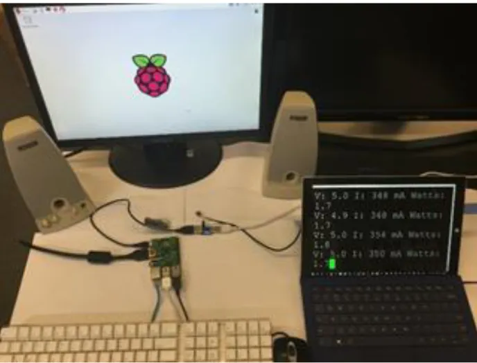
We used the following hardware as shown in Figure 3.1: Raspberry Pi B+, 1080p monitor,
Adafruit USB Power Gauge A/D converter (Power Gauge), keyboard, mouse, speaker, and
Ethernet.
The Power Gauge is a micro-board that can measure the voltage and current. It has several LED
lights on board that shows the output power at the rate of about 1.5s. Its LED lights are indicators
of the instantaneous power and are accurate to 0.1 Watts. Additionally, it has a USB serial port
that can transmit the voltage, current, and power usage message to another computer. The Power
Gauge should be connected to the power supply with the input port, and the output port with the
power port of the RPI, and plug the additional serial USB port to another computer.
In a Windows machine, it is recommended to use putty serial port connection to read the serial
port data. We used the Device Manager to find the USB port serial line that was currently
12
Figure 3.1 Whole experimental setup
3.2.2 Software
We used the following software: System: Raspbian, Performance counters: Perf, System
monitor: Top, SSH(Secure Shell), Serial connection software: putty, Benchmarks: OMXplayer,
Mplayer, VLC player, 3D-slash
3.2.2.1 Performance counters: Perf
Perf is a tool that uses performance counters in Linux. Performance counters are CPU hardware
13
can output the instructions and cycles that the CPU has executed. In our research, we used Perf
to access the counters before and after each benchmark.
3.2.2.2 System monitor: Top
Top is a system monitor that can watch the system load. Its refresh rate can vary. It can read the
CPU and Memory use rate, but it cannot read the GPU use rate. For RPI, its GPU chip has been
recently supported by OpenGL, and it hasn’t had a direct GPU monitor yet. In this research, we
were using remote SSH connection with RPI, and ran TOP on a remote desktop to avoid
unnecessary GPU operation on RPI that may increase the energy consumption.
3.2.2.3 Benchmarks:
Benchmarks are the software used to test performance. In this research, we focused on
benchmarks that exercise the GPU.
3.2.2.3.1 OMXplayer
OMXplayer is a built-in video player that comes with the Raspbian system, and it is specifically
made for the RPI’s GPU. It relies on the OpenMAX hardware acceleration API, which is the
Broadcom's VideoCore officially supported API for GPU video/audio processing [20]. It is a
very small program and has OpenGL support and GPU rendering on the RPI. The OMXplayer
does not have graphical user interface but is controlled by key bindings. It is capable of playing
MP4, MP3, and MKV [21].
3.2.2.3.2 Mplayer
Mplayer is available in the Linux APT (Advanced Packaging Tool) library. It is also very
14
3.2.2.3.3 VLC player
VLC player is relatively bigger than the OMXplayer and the Mplayer. It has a graphical user
interface (GUI) and does not have GPU rendering support on the RPI.
3.2.2.3.4 3D-slash
3D-slash is a 3D modeling program that allows the user to modify 3D models. It has GPU
rendering support and uses a considerable amount of RAM. To use it, the user must allocate
more RAM for GPU after installation. It has EGL (Embedded-System Graphics Library) [22]
and GLES (OpenGL for Embedded Systems) support [23].
3.2.2.4 Putty
The Putty is a tool that allows SSH or serial port connection with Linux machines. Our research
used both remote SSH desktop and serial port connection. The SSH was used to log in to the
RPI, while the serial port was used for the PC to receive data from the serial port of the power
15
Figure 3.2 Putty setup for serial port recording.
3.3 GATHERING DATA
3.3.1 Perf
The following is a representative use of Perf command ($sudo perf_3.16 stat -e
instructions,cycles omxplayer ~/video file name), sudo -- we need sudo for security/permissions
reasons (we could have instead set the perf_event_paranoid valid). For perf_3.16, we specify a
version number due to how the Linux developers ship perf with the kernel source code. Even
though it is usually backwards compatible, the Debian setup always tries to use a version
16
This command lets Perf access the performance counters when OMXplayer renders a video file
and display the instructions and cycles after the program completes. Then the instructions per
cycle can be calculated. The more data the CPU processes, the higher the instructions per cycle
value.
3.3.2 Putty
3.3.2.1 Adafruit USB Power Gauge A/D converter
We used putty to output a log file that records the real-time Adafruit USB Power Gauge A/D
converter data. After we got the log file, we used a script to post-process it to get the voltage and
current and calculate the power.
3.3.2.2 Top
We used Top running on RPI in the background using a remote SSH connection to capture CPU
and memory usage. We logged this output to a file with the following command ($top –b n30
|grep omxplayer > omxplayer_top)
This command recorded 30 updates of the Top output (approximately 60 seconds) and captured
the OMXplayer CPU and memory usage of the system.
3.4 RESULTS
We ran the benchmarks and used the tools to assess the performance. We used Top to measure
CPU and memory usage, Perf to measure the number of cycles per instruction, and the Power
Gauge to measure voltage and current (and therefore power). The results from Top that
17
3.4, and the power results are shown in Figure 3.5, Figure 3.6, and Figure 3.7. The energy
comparison between OMXplayer and Mplayer is shown in Figure 3.8.
18
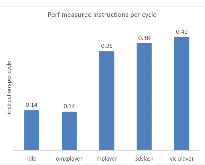
Figure 3.4 Instructions per cycle under different benchmarks
3.4.1 OMXplayer
OMXplayer is a built-in primary video player and is included with Raspbian. It is made
explicitly for the RPI's GPU and uses little CPU and memory. With fast response speed and
smoothness, it is highly recommended on Raspberry Pi. The results measured by Top showed
CPU usage to be 18% and memory use at 7%. Perf reported the instructions per cycle to be 0.14
(virtually identical to idle), and the average power for the run was 1.92W. The total run time
19
3.4.2 Mplayer
We tested the Mplayer; it played the video at a frame rate of 1fps. It did not drop frames;
however, it simply played too slowly. It used no hardware acceleration and reported: "Your
system is too slow to play this.". Top measured: CPU use: 86% and memory use: 18%. Perf
reported the instructions per cycle to be 0.35 (indicating higher CPU usage compared to idle),
and the average power for the run was 1.89W. The total run time was approximately 10 minutes.
3.4.3 VLC player
VLC player ran poorly on the RPI. Its frame rate was 0.01fps. The VLC player was not hardware
accelerated. The results measured by Top were CPU 78% and memory use 28%. Perf reported
the instructions per cycle to be 0.4 and the average power for the ran was 1.87W. Due to the
prolonged frame rate the video was stopped before it finished.
3.4.4 3D-slash
Although 3D-slash is not a video player, we assessed its performance in manipulating 3D
models. We modified non-HD models and got the following performance values: Top measured
CPU 52% and memory use 42%, Perf reported the instructions per cycle to be 0.38, and the
20
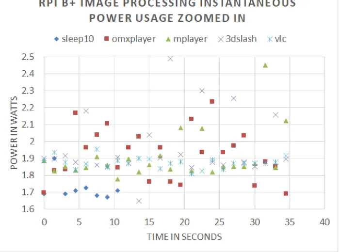
Figure 3.5 Power vs time for each benchmark.
3.4.5 Discussion
Looking at the instructions per cycle data in Figure 3.4, we can see that with idle and the
OMXplayer the instructions per cycle was lower than Mplayer, 3D-slash, and VLC player. This
means that the OMXplayer had relatively fewer instructions processed by the CPU compared to
Mplayer, 3D-slash and VLC player. OMXplayer used hardware rendering while Mplayer and
VLC player did not which resulted in the higher instructions per cycle value. Since 3D-slash
21
were high. The memory usage of 3D-slash was the highest, the VLC player used more memory
than Mplayer, which in turn used more memory than OMXplayer.
In Figure 3.5, the more time the benchmarks uses to render the video file, the Power Gauge
would draw more sample points. Omxplayer had the least sample points, while mplayer had
more sample points and VLC couldn't finish playing the video so it was cut off in the middle.
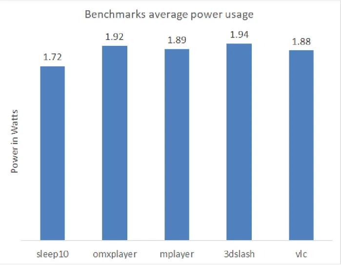
One can see in Figure 3.7 that there was a power penalty when using the GPU as the power
consumption by 3D-slash(1.94w) and OMXplayer(1.92w) was noticeably higher than the VLC
player(1.87w) and Mplayer(1.88w). Not surprisingly, all of the programs had significantly
higher power than an idle board(1.72w). One important consideration, however, was that even
though the power consumption was lower for Mplayer than for OMXplayer, the time to render
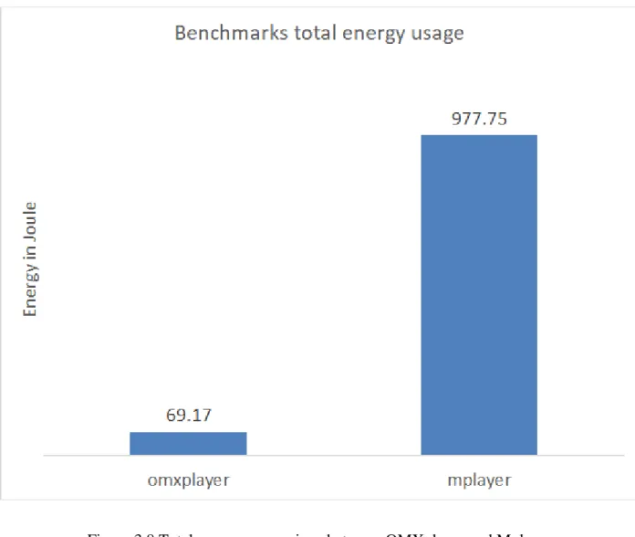
the whole video was considerably longer. Thus, although the power was higher when the
OMXplayer was used, the total energy to play the video was about 14 times less (see Figure 3.8)
than for Mplayer. The VLC player had such a poor performance that the total energy calculation
could not be done, but would have been approximately 100 times higher than Mplayer. This ratio
result was an unusual circumstance as the higher performance solution (OMXplayer), that used
more power, ultimately used significantly less energy since it accomplished in 30 seconds what
22
23
24
Figure 3.8 Total energy comparison between OMXplayer and Mplayer
3.5 CONCLUSION AND FUTURE WORK
From this research, we have shown that RPI with the GPU rendering had a significantly better
performance than the software rendering. Hardware rendering used more power than the software rendering. However, hardware rendering’s total energy efficiency can be higher than
the software rendering’s because of the extended time that was taken by software rendering. We
tested several video playing applications as well as a 3D modeling program. Those that used
25
used hardware rendering used more power but performed significantly better regarding rendering
speed. Given that there was no GPU monitor for the RPI we inferred the GPU contribution and
power draw using putty, Perf, Top, Power Gauge and wrote scripts to post-process the log files.
RPI is a low power consumption microcomputer and studying its graphical performance and its
power efficiency is vital in making intelligent design decisions where energy was limited.
We found some limits in monitoring the system information about the GPU and the shared RAM between CPU and GPU. With OpenGL supporting the RPI’s graphics card, more graphics
monitor programs could be written, as well as more power measure methods and additional
26
4. COMPARING POWER AND ENERGY USAGE FOR SCIENTIFIC CALCULATION
WITH AND WITHOUT GPU ACCELERATION ON A RASPBERRY PI MODEL B+
AND 3B
4.1 INTRODUCTION
In this work, we sought to quantify and compare the energy and power usage of a small,
low-power, single board computer, specifically the Raspberry Pi. The Raspberry Pi is a board that can
be purchased for under $50 and contains a Graphics Processing Unit (GPU) as well as the
Central Processing Unit (CPU). We were interested in comparing power and energy
consumption when performing an intensive calculation utilizing the GPU vs. the same
calculation using only the CPU. The algorithm chosen was the Fast Fourier Transform (FFT) for
a variety of input data set sizes. The FFT method used in Digital Signal Processing (DSP) was
included in the top 10 algorithms of the 20th century by the IEEE journal Computing in Science
& Engineering [12].
Digital devices are pervasive in our lives. If a high-quality audio clip plays on a Bluetooth
headphone, the delay-time of the transmitting audio signal is ideally shorter and the battery life
should be longer. Also, the quality of sound is better with a higher sampling rate and with more
bits of precision. Thus, there is a desire to be able to quickly complete the most calculations
possible using the least total energy (battery life).
The use of GPGPU code is suitable when processing massive data. GPGPU code can run using
the GPU on RPIs for processing large data. To find out the elapsed time, power, and energy
usage, we wrote six benchmarks that use three libraries: GPU_FFT for RPIs in C [1], FFTW in C
27
these libraries to process single-precision floating point data. GPU_FFT used GPGPU code,
FFTW used the serial code in C, and SciPy FFT used the serial code in Python to compute FFT.
Then, the runtimes of the benchmarks were measured by their built-in time counter. Externally, the Power Gauge measured the test device RPIs’ power and energy.
Before we considered this topic, we studied the power and energy usage of the RPI B+ when it
played a short video using CPU and GPU [16]. We found that utilizing the GPU for video
rendering not only greatly improved the video performance but also decreased the total energy
used in rendering the video.
We leveraged code for the Raspberry Pi that utilized the GPU for FFT calculation. The code,
GPU_FFT, could be downloaded from GitHub [1]. Computing FFT with a microcontroller was
not unique to a Raspberry Pi. There are other FFT implementations on DSP models: TMS320
chips have FFT accelerators that promised excellent performance in DSP [24]. Despite this, if we
were looking for a multimedia board that was capable of processing DSP while also functioning
as a general-purpose Linux computer, RPIs were an excellent choice. This study will advance
our understanding of how the utilization of the GPU for significant throughput data affects
speed, energy efficiency.
4.2 EXPERIMENTAL SETUP
The experiment setup includes hardware and software setup.
4.2.1 Hardware
In this section, we are going to cover the hardware equipments and the hardware parameter
28
4.2.1.1 Hardware specifics
There were some hardware upgrades from RPI B+ to RPI 3B. In our experiment, we mainly
focused on the performance of the benchmarks on CPU, GPU, and we listed them in Table 4.1.
RPI SoC CPU GPU Memory
(SDRAM) B+ Broadcom BCM2835 700 MHz 32-bit single-core ARM, Arm1176JZ(F)-S Broadcom VideoCore IV @ 250 MHz, OpenGL ES 2.0 (24 GFLOPS) 512 MB (shared with GPU) 3B Broadcom BCM2837 1.2 GHz 64-bit quad-core ARM, Cortex-A53 (ARMv8) cluster, NEON. 3D part of GPU @ 300 MHz,
video part of GPU @ 400 MHz,
OpenGL ES 2.0 (28.8 GFLOPS)
1 GB
(shared
with GPU)
Table 4.1 RPI B+ and 3B Key Hardware Information
The hardware for the experimental setup consisted of the RPI B+ and RPI 3B under test and an
Adafruit USB Power Gauge. The Power Gauge had its majority power measurement acquired
from an INA210 high side current sensor to measure the current on each line broken out by the
interceptor boards [19]. The INA219 could measure up to 3.2A of current with a resolution of
0.8mA. The Power Gauge was connected between the power source and the RPIs power input. It
29
connected to the host machine it presented itself as a serial port over which the data was
transferred. We used a Linux machine and Minicom software for capturing the logged data.
Figure 4.1 Hardware and Software setups
Figure 4.1 shows one of the benchmarks running and logging the voltage, current, and power.
After we measured the power by Power Gauge, we tried to measure the power with a higher
sample rate (for 4 seconds time span, we used 1 KHz sampling rate), higher voltage precision
using Analog discovery 2 Digilent to prove the results are correct. Digilent needed a external
30
measured 1D FFT on RPI 3B for single run for comparing the results with Power Gauge
measured results. Then we used the software Waveforms to output the sample points to CSV file.
Figure 4.2 shows the RPI external circuit for powering and measuring power of the RPI.
Figure 4.2 RPI external circuit for powering and measuring power
4.2.1.2 Hardware System Settings
4.2.1.2.1 Memory Split
RAM (Random Access Memory) on RPI B+ and RPI 3B is shared by their CPUs and GPUs. We
could allocate GPU_RAM customized in the command ($sudo raspi-config) under category
Advanced Options, Memory Split. We needed to allocate more GPU_RAM when GPU_FFT was
processing large FFT_length 1D and 2D FFT, and we needed to allocate less GPU_RAM when
31
setting the GPU_RAM was 16MB MIN (minimum), MAX (maximum) was depending on
different RPI models. In our experiments, we used the command ($watch -n 1 free -h) to watch
the system RAM usage. We got our RAM usage of the 6 benchmarks by subtracting RAM usage
to idle. We set the benchmarks to do 1D FFT at a FFT_length of 2^22 and looped for 40 times,
and then did 2D FFT at a FFT_length of 2^11 and looped for 20 times. In Figure 4.3, it showed
the GPU_RAM and CPU_RAM needed for each benchmark to run a maximum FFT_length and
loops.
32
4.2.1.2.2 V3D with OpenGL ES
V3D must be enabled to run concurrently with the OpenGL ES when GPU_FFT is started [1].
The V3D was enabled using the command ($sudo raspi-config) under category Advanced
Options, GL Driver, G3 Legacy. This GL Driver toggle switch was only enabled after RPI model
2. There is a special case for RPI B+: The installation guide for GPU_FFT on RPI B+ must be
followed because RPI B+ could not toggle GL options as mentioned. Installation command was
($sudo apt-get install gpu-fft && sudo rpi-update && sudo reboot).
4.2.2 Software
The only key software on the data gathering machine was Minicom that was used to capture the
data in CSV files. The Raspberry Pi ran the Raspbian operating system. Connections were made
using SSH. We used the GPU_FFT library with the included "hello_fft" program to calculate the
FFT in 1D and 2D [1]. We used Python version 2.7 with the SciPy and NumPy libraries with
Python code that we developed using those libraries for computing the FFT in 1D and 2D [3].
Finally, we used the FFTW library and C code that we developed to also compute the FFT in 1D
and 2D [2]. All FFT results were compared to the known correct values to verify the code.
4.2.2.1 Minicom
We set up Minicom for the logging of the power data points. We set a particular USB port that
Power Gauge logs data to in Minicom settings. Then we ran Minicom and captured the recorded
data to a text file as we did in Figure 4.1. In the end, we used Microsoft Office Excel to import
33
4.2.2.2 Input Settings
In the 1D IFFT input array, we set the N input elements in a row array, where log2_N increased
from 8 to 22. Therefore, the number of elements varied from 2^8 to 2^22. To generate a result
that has a known exact solution, we set the input to be the FFT of a cosine function. Based on the
known answer, we were able to get the REL_RMS_ERR by comparing the output with the
known solution. In the testing, we had found that SciPy.fftpack had mistakenly confused the
IFFT and FFT functions. When SciPy.fftpack was used to call the FFT function, a IFFT function
was called instead and vice versa.
In the 2D FFT input array, we set the N*N elements in a matrix. The input matrix varies with the
following measurements: 2^16, 2^18, 2^20, 2^22. We set the coordinate (0,0) value to be 1. This
is a Dirac delta function. In a DFT that has finite sample points, it will produce a result of all
ones in the output. This Dirac delta function is considerably beneficial for the checking
REL_RMS_ERR for simplifying the exact solution.
4.2.2.3 Timing, REL_RMS_ERR, and Others
We used command line arguments in the benchmarks scripts that allowed selecting specific FFT
length range, loop times, option to skip REL_RMS_ERR, option to skip output Bitmap Image
File (BMP).
The benchmarks looped through different job sizes and got us a broad view of the libraries
performances. When using the timing libraries that were built-in in C and Python languages, we
considered the resolution of the time() function. So we checked the overhead of the function by
running the time() function several times and printed out the time() values. Many dry run results
34
time() function for details checking each part of the FFT process, including initializing the input
in every loop, calling for FFT function, and calculating REL_RMS_ERR.
We considered wrapping the order of the loops for code efficiency. The outside loop was looping
through the FFT_length from small to big; then in the inside loop, we ran the assigned
FFT_length many times. This wrapping order would match more of the prediction of the CPU
cache, producing fewer cache misses and making the runtime shorter.
We also had switches for REL_RMS_ERR to check for the first few runs to debug the program
and performance accuracy resolution check since the REL_RMS_ERR was taking much more
time than the FFT process time.
In the 2D FFT, GPU_FFT could produce an output BMP file. In the debugging section, we used
the image for checking error in addition to the REL_RMS_ERR.
The comparison of RPI B+ and 3B running the same 6 benchmarks will give us a more objective
view of how the similar, but upgraded microcomputer board affects the libraries performance.
4.3 RESULTS
This section discusses the results that were obtained. The following time elapsed images are
log/log scaled. On the Y label, time is also logarithmic.
4.3.1 Benchmarks 1D and 2D FFT Time Elapsed
The first criteria was the time that was required for the calculation to be completed. The
following figures show the times for the 1D and the 2D FFT calculations.
In Figure 4.4, and Figure 4.5, the 1D FFT on RPI B+ and 3B, we can see that as the job size
35
FFTW is about 10x slower compared with the speed of GPU_FFT, whereas SciPy FFT’s speed is
around 15x slower than GPU_FFT’s. On RPI 3B, the speed of FFTW is about 2.8x slower
compared with the speed of GPU_FFT, whereas SciPy FFT’s speed is around 3.7x slower than GPU_FFT’s.
In Figure 4.6, and Figure 4.7, the 2D FFT on RPI B+ and 3B, we can see the pattern is similar to
the pattern in Figure 4.4 and Figure 4.5. On RPI B+, FFTW and SciPy FFT are about 10x slower
than GPU_FFT. However, SciPy FFT is taking less time than FFTW. On RPI B+, when running
2D FFT, FFTW is not as good as SciPy FFT in speed, and the best is still GPU_FFT, which is
roughly 10x faster. On RPI 3B, when running 2D FFT, FFTW is about 6x slower than
36
37
Figure 4.5 1D FFT RPI 3B time (in seconds) elapsed for each of the 3 libraries
Figure 4.8 shows us the output BMP file of 2D FFT. Using the 2D FFT output image can make
FFT easier to visualize and understand. The BMP file pixel values are not easy to verify by
checking the file. We eventually checked the output values by comparing all the pixel values to 1
to get REL_RMS_ERR.
In the GPU_FFT library, there was a function that could set batches to more than one batch that
produced more throughput for the GPU. The library manual said it would trim down the time for
38
extended as we increased the batch size. In our experiments, we always set the batch size to be 1
to get the best performance.
39
Figure 4.7 2D FFT RPI 3B time (in seconds) elapsed for the 3 libraries
40
4.3.2 Power and Energy
As was stated earlier, the speed of a calculation is important, especially for embedded devices.
The power consumption and energy consumption are also important factors. Energy usage is of
particular importance in battery-powered applications as a battery is essentially capable of
delivering a particular amount of energy.
In Figure 4.9, and Figure 4.10, power measure of running 1D FFT on RPI B+ and 3B, we have
the GPU_FFT, FFTW and SciPy FFT have different amounts of sample points. The sample
points resolution is about 40 samples per minute [19]. GPU_FFT and FFTW run faster than
SciPy FFT, so GPU_FFT and FFTW have the smallest amount and the second smallest amount
of sample points, respectively. On RPI B+, the power consumption running FFTW and SciPy
FFT reach their peak at just over 2W; however, the highest power usage is the GPU_FFT, and it
reaches up to 2.1W maximum when calculating the 1D FFT. SciPy FFT and FFTW have about
the same power usage as one another and less than the GPU_FFT. On RPI 3B board, SciPy FFT
and FFTW are taking the most power peak at 4W and the second most power peak at 3.5W,
41
Figure 4.9 Instantaneous power comparison of 3 libraries process 1D FFT 40 loops of
42
Figure 4.10 Instantaneous power comparison of 3 libraries process 1D FFT 40 loops of
FFT_length 2^22 on RPI 3B
In Figure 4.11, it’s Digilent measured power of RPI 3B doing 1D FFT for a single run. The
power data points are very similar with the Power Gauge measured in Figure 4.10. That proves
43
Figure 4.11 Digilent measured RPI 3B 1D FFT instantaneous power usage
In Figure 4.12, and Figure 4.13, 2D FFT on RPI B+ and 3B, the pattern is similar with the 1D
FFT on 2 different boards. On RPI B+, the power consumption is led by GPU_FFT that has its
power peak at 2.2W, FFTW and SciPy FFT have their peak around 1.8W. On RPI 3B, FFTW
44
Figure 4.12 Instantaneous power comparison of 3 libraries process 2D FFT 20 loops of
45
Figure 4.13 Instantaneous power comparison of 3 libraries process 2D FFT 20 loops of
FFT_length 2^11 on RPI 3B
In Figure 4.14, we calculated the sum of the data points from Figure 4.9, Figure 4.10, Figure
4.12, and Figure 4.13 and generated the energy usage graph. In Figure 4.14, 1D FFT part, we can
see GPU_FFT is using the least total energy whether on RPI B+ or 3B among 3 libraries. When
doing 1D FFT on RPI B+, the power is higher (2.1W) when doing GPU_FFT than the other two
libraries (1.8W), but the time for processing makes up the disadvantage and makes its total energy less than the other two libraries’.
46
47
48
49
50
Figure 4.18 Power Gauge measured RPI 3B 1DFFT energy usage
When doing 1D FFT on RPI 3B, the power is lower when doing GPU_FFT (2.8W) than the
other two libraries (FFTW 3.1W, SciPy FFT 3.8W) and its time for processing is shorter than the
other libraries. Therefore, GPU_FFT on RPI 3B uses less energy than the other two libraries. In
Figure 4.14, 2D FFT part, it shows that GPU_FFT is using the least total energy whether on RPI
B+ or 3B among 3 libraries. When doing 2D FFT on RPI B+, the power is higher when doing GPU_FFT (2W) than the other two libraries (FFTW, SciPy FFT 1.7W), but GPU_FFT’s less
processing time makes up for the disadvantage and causes its total energy to be less than the other two libraries’. The power on RPI 3B is significantly higher for FFTW (3W) and SciPy FFT
51
(3.3W) when doing 2D FFT, and their powers are higher than GPU_FFT’s power (2.6W).
GPU_FFT still runs faster than the other two libraries on RPI 3B, so the GPU_FFT's total energy
is lower because the GPU_FFT also uses less power. In 2D FFT, SciPy FFT takes less time and
less energy than FFTW on both RPI B+ and 3B.
In 1D, 2D FFT, the upgrade of RPI B+ to 3B have reduced the energy usage of FFTW and SciPy
FFT more than 50% by powering up and reducing the processing time. However, the increase in
power feeding for CPU and GPU on RPI 3B also causes GPU_FFT on RPI 3B uses more energy
than on RPI B+ since the time elapsed for GPU_FFT has not significantly shortened to make up
the disadvantage in the higher power usage. Overall, whether on RPI 3B or B+, using the
GPU_FFT to calculate the FFT uses less than 2/3 to 1/3 of the energy of any other method of
computing the FFT.
In Figure 4.15, and Figure 4.16, 1D and 2D FFT Energy-Delay values are compared. The
Energy-Delay values of GPU_FFT are the smallest in 1D and 2D FFT, and that is less than 1/2 of other libraries’ Energy-Delay values on both RPI B+ and 3B.
In Figure 4.17, and Figure 4.18, Digilent and Power Gauge measured energy usage per run when
running 1D FFT at FFT_length equals to 2^22, We can see that FFTW and GPU_FFT energy
usage are very similar on both graphs. The SciPy FFT energy usage is higher in Digilent than in
Power Gauge because when using Digilent to measure, we have single run that has overhead.
When we use the Power Gauge to measure, we have multiple runs that average values brings
52
4.3.3 Total Time and Init-Time
The previous sections focused on the time to do the FFT calculations; however, the FFT requires
setting up the input buffer, which requires a non-trivial amount of time. We measured this
initialization time as well as the time to calculate the error in the calculation.
Figure 4.19, Figure 4.20 shows the 1D FFT initializing time elapsed on RPI B+, 3B. Figure 4.21,
Figure 4.22 shows the 2D FFT initializing time elapsed on RPI B+, 3B. Though in 3 libraries, the
initializing array does not has a GPU rendering support, it’s all CPU processed. Its time elapsed a
significant portion of the total time elapsed. We can see FFTW performs very well when the
FFT_length is small, as the FFT_ length increases to 2^22, the GPU_FFT has the greatest time
elapsed, about 1000X more than SciPy FFT on RPI B+, and more than 5000X on RPI 3B. Scipy
FFT has the smallest time usage. FFTW is in the middle, about 1000X more than SciPy FFT on
RPI B+ and 3B. We can see that in 2D FFT, as the FFT_ length increases to 2^22, the GPU_FFT
has the greatest time elapsed, about 1000x more than SciPy FFT on RPI B+, over 5000x more
than SciPy FFT on RPI 3B. FFTW is in the middle, about 1000x more than SciPy on RPI B+,
53
54
55
56
57
58
Figure 4.24 2D FFT total time compare of 3 libraries on RPI B+ and RPI 3B
In Figure 4.23, we have the total time comparison of the 1D FFT, FFT_length 2^22 of 3 libraries
on RPI B+ and 3B. On RPI B+, the total time ranking for the 3 libraries order from greatest to
smallest is: SciPy FFT, FFTW, and GPU_FFT. FFTW has a bigger portion of initializing time when compared with SciPy FFT’s. GPU_FFT has the greatest portion of initializing time of the 3
libraries. However, FFTW and GPU_FFT have shorter FFT time that make over the
disadvantage in INIT-time and caused the total time to be less than SciPy FFT’s total time.
Python is good at allocating memory, and that benefits the SciPy to have less Init-time. On RPI
59
RPI 3B the FFTW is the second fastest and takes more than 2 seconds for the total time but is
still slower than GPU_FFT and runs the same job on RPI B+ in less than 2 seconds.
In Figure 4.24, we have the total time comparison of the 2D FFT, FFT_length 2^11 of 3 libraries
on RPI B+ and 3B. On RPI B+, the pattern is similar to the Figure 4.23, but the SciPy FFT is
faster than FFTW in 2D FFT, so we have the total time rankings from least to greatest as GPU_FFT, SciPy FFT, and FFTW. FFTW’s total time has a larger portion of initializing time
compare with SciPy FFT’s. GPU_FFT’s total time has the largest portion of Init-time in the 3
libraries. 2D FFT have bigger matrices that need to be initialized. The RPI 3B has the same
pattern, where SciPy FFT (less than 2s) on RPI 3B is taken little time but still requires more time
than GPU_FFT on RPI B+ and also on RPI 3B.
4.3.4 REL_RMS_ERR Value
In this section, we discuss the error in the FFT calculation. We calculated the relative root mean
60
0000
Figure 4.25 REL_RMS_ERR comparison of 3 libraries process 1D FFT
In Figure 4.25, FFTW shows the least REL_RMS_ERR, SciPy FFT has the second least
REL_RMS_ERR, and GPU_FFT has the highest REL_RMS_ERR. The REL_RMS_ERR range
is from 1e-5 to 1e-8. When considering the scale of the error, the REL_RMS_ERR is at a level of
1 parts per million or less This precision would satisfy most daily needs.
4.4 CONCLUSION AND FUTURE WORK
By comparing the FFT elapsed time, total time, power and energy consumption of six
61
processes large data throughput FFT arrays quickly and as the FFT length size increases, the
speedup is easier to see. This speedup does not sacrifice too much precision in REL_RMS_ERR.
Also, it benefits the energy efficiency because even though it consumes more power for
computing when we are running benchmarks on the single core RPI B+, the significant speed
increase results in less total energy usage and less energy delay. When we have the benchmarks
running quad-core RPI 3B with faster CPU and GPU, the speed up of the serial code is
tremendous, and it does save energy by reducing the computing time; however, on RPI 3B, the
power feed for the CPU is greater than the feed for GPU, so RPI 3B still needs more power and
more energy to process serial code than parallel code. Nevertheless, GPU_FFT runs on RPI B+,
and 3B are still faster and take less energy than FFTW and SciPy FFT run on RPI 3B. Generally
speaking, the GPU_FFT library is a successful library that runs FFT on RPIs with excellent
accuracy, fast speed, and greater energy efficiency compared with other FFTW and
SciPy.fftpack libraries. In the future study, we might follow the pattern and study more about
parallel programming including MPI, CUDA, power, energy implication and apply it on a
62
5. RESULTS, CONCLUSION, AND FUTURE WORK
The first study was performed on Raspberry Pi model B+. We managed to quantify the different video player benchmarks’ (the OMXplayer, 3D slash with, and the Mplayer, the VLC player
without GPU rendering) performance when they were handling the same job and correlate their
frame rendering performance with their power and energy performance. We also had a 3D model
simulator running for power and energy comparison. We used various system tools to read the
system details. The results showed that the benchmarks OMXplayer with GPU rendering had a
visible difference in power consumption higher than the benchmarks the Mplayer, the VLC
player without GPU rendering. However, the process time for the same job size process by
benchmark with GPU rendering was significantly shorter than the benchmarks without GPU
rendering. The time difference had made up for the disadvantage in higher power usage and
made the benchmark with GPU rendering more power efficient.
The second study was conducted on the Raspberry Pi model B+ and 3B. We ran comparisons
between 3 libraries doing a scientific calculation using complex values. The DSP method we
used in the three libraries was the FFT. The calculations were in both 1D and 2D. We had the
single precision floating point numbers set as the primary data type. Also, we correlated the
performance of the benchmarks (GPU_FFT with GPU render, and FFTW, SciPy.FFT without
GPU rendering) speed, accuracy, power, and energy. On both RPI models, the results showed the
benchmark GPU_FFT with GPU rendering took less energy than the other benchmarks without
GPU rendering. On RPI B+, GPU_FFT used more power, less time, and less total energy than
the FFTW, SciPy.FFT libraries. On RPI 3B, GPU_FFT used less power, and less time, and less
63
In this thesis, we found that on a small single-board computer Raspberry Pi, in some fields like
processing video files, processing 3D models, and calculating complex values using a scientific
method, using a GPU rendering significantly shortens the process time and also saves energy.
We interpret that using GPU for rendering in some suitable fields that required multiple threads
doing the same instructions are fast and energy efficient.
The results described in this thesis are highly intriguing in that repeatedly, we found
circumstances in which the fastest processing also consumed the least total energy. For the
Raspberry Pi model B+, the method that used the least total energy consumed the most power
(but for a much shorter time). For the Raspberry Pi model 3B, however, when performing FFT
calculations the GPU used less total energy, finished computing in less time, and consumed less
power while the computation was occuring.
We find these results on the RPI very interesting and hypothesize that similar testing on CUDA
or more massive machines in the future may yield comparable results. Further work may include
a double precision calculation on the RPI GPU. It may also include different benchmarks that
implement the looping order inside the function differently to test the cache misses penalty on
64
REFERENCES
[1] Holme, A. (n.d.). GPU_FFT. Retrieved April 05, 2018, from
http://www.aholme.co.uk/GPU_FFT/Main.htm
[2] Frigo, M., & Johnson, S. G. (n.d.). FFTW Home Page. Retrieved April 05, 2018, from
http://www.fftw.org/
[3] Discrete Fourier transforms (scipy.fftpack). (n.d.). Retrieved April 05, 2018, from
https://docs.scipy.org/doc/scipy/reference/fftpack.html
[4] Singer, G. (2013, March 27). The History of the Modern Graphics Processor. Retrieved
April 05, 2018, from https://www.techspot.com/article/650-history-of-the-gpu/
[5] Graphics processing unit. (2018, April 04). Retrieved April 05, 2018, from
https://en.wikipedia.org/wiki/Graphics_processing_unit
[6] Hardware acceleration. (2018, April 04). Retrieved April 05, 2018, from
https://en.wikipedia.org/wiki/Hardware_acceleration
[7] General-purpose computing on graphics processing units. (2018, April 03). Retrieved
April 05, 2018, from
https://en.wikipedia.org/wiki/General-purpose_computing_on_graphics_processing_units
[8] Raspberry Pi. (2018, April 05). Retrieved April 05, 2018, from
https://en.wikipedia.org/wiki/Raspberry_Pi
[9] Kerin, A. (2014, June 13). Power vs. Performance Management of the CPU. Retrieved
April 05, 2018, from
65
[10] Wulf, W. A., & McKee, S. A. (1995, March). Hitting the memory wall: Implications of
the obvious. Retrieved April 05, 2018, from https://dl.acm.org/citation.cfm?id=216588
[11] Schaller, R. R. (1997, June). Moore's law: Past, present and future. Retrieved April 10,
2018, from https://ieeexplore-ieee-org.prxy4.ursus.maine.edu/abstract/document/591665/
[12] Dongarra, J., & Sullivan, F. (2000, January). Guest Editors Introduction to the top 10
algorithms. Retrieved April 05, 2018, from http://ieeexplore.ieee.org/document/814652/
[13] Hanada, T., Sasaki, H., Inoue, K., & Murakami, K. (2012, August). Performance
evaluation of 3D stacked multi-core processors with temperature consideration. Retrieved April
05, 2018, from http://ieeexplore.ieee.org/document/6263025/
[14] Jiao, Y., Lin, H., Balaji, P., & Feng, W. (2011, March 07). Power and Performance
Characterization of Computational Kernels on the GPU. Retrieved April 05, 2018, from
http://ieeexplore.ieee.org/document/5724833/
[15] Sabarinath, S., Shyam, R., Aneesh, C., Gandhiraj, R., & Soman, K. P. (2015, Spring).
Accelerated FFT computation for GNU radio using GPU of raspberry Pi. Retrieved April 05,
2018, from
https://www.amrita.edu/publication/accelerated-fft-computation-gnu-radio-using-gpu-raspberry-pi
[16] He, Q., Segee, B., & Weaver, V. (2017, March 20). Raspberry Pi 2 B GPU Power,
Performance, and Energy Implications. Retrieved April 05, 2018, from