Automatic model selection for partially linear models

Contents lists available atScienceDirect

Journal of Multivariate Analysis

journal homepage:www.elsevier.com/locate/jmva

Automatic model selection for partially linear models

Xiao Ni, Hao Helen Zhang

∗

, Daowen Zhang

Department of Statistics, North Carolina State University, United States

a r t i c l e i n f o Article history:

Received 8 January 2008 Available online 25 June 2009 AMS subject classification: 62G08

62J07 Keywords:

Semiparametric regression Smoothing splines

Smoothly clipped absolute deviation Variable selection

a b s t r a c t

We propose and study a unified procedure for variable selection in partially linear models. A new type of double-penalized least squares is formulated, using the smoothing spline to estimate the nonparametric part and applying a shrinkage penalty on parametric components to achieve model parsimony. Theoretically we show that, with proper choices of the smoothing and regularization parameters, the proposed procedure can be as efficient as the oracle estimator [J. Fan, R. Li, Variable selection via nonconcave penalized likelihood and its oracle properties, Journal of American Statistical Association 96 (2001) 1348–1360]. We also study the asymptotic properties of the estimator when the number of parametric effects diverges with the sample size. Frequentist and Bayesian estimates of the covariance and confidence intervals are derived for the estimators. One great advantage of this procedure is its linear mixed model (LMM) representation, which greatly facilitates its implementation by using standard statistical software. Furthermore, the LMM framework enables one to treat the smoothing parameter as a variance component and hence conveniently estimate it together with other regression coefficients. Extensive numerical studies are conducted to demonstrate the effective performance of the proposed procedure.

©2009 Elsevier Inc. All rights reserved.

1. Introduction

Partially linear models are popular semiparametric modeling techniques which assume the mean response of interest to be linearly dependent on some covariates, whereas its relation to other additional variables are characterized by nonparametric functions. In particular, we consider a partially linear modelY

=

XT

β

+

f

(

T

)

+

ε

, whereXare explanatory variables of primary interest,

β

are regression parameters,f

(

·

)

is an unknown smooth function of the auxiliary covariateT, and the errors are uncorrelated. This model is a special case of general additive models [1]. Estimation of

β

andf has been studied in various contexts including kernel smoothing [2], smoothing splines [3–7], and penalized splines [8,9].

Often times, the number of potential explanatory variables,d, is large, but only a subset of them are predictive to the response. Variable selection is necessary to improve prediction accuracy and model interpretability of final models. In this paper, we treatf

(

T

)

as a nuisance effect and mainly focus on automatic selection, estimation and inferences for important linear effects in the presence ofT. For linear models, numerous variable selection methods have been developed such as stepwise selection, best subset selection, and shrinkage methods like nonnegative garrote [10], least absolute selection and shrinkage operator (LASSO; [11]), smoothly clipped absolute deviation (SCAD; [12]), least angle regression [13], adaptive lasso [14,15]. Information criteria commonly used for model comparison include MallowsCp [16], Akaike’s Information

Criteria [17] and Bayesian Information Criteria (BIC; [18]). A thorough review on variable selection for linear models is given in [19,20].

∗_{Corresponding address: Department of Statistics, North Carolina State University, Campus Box 8203, 27695-8203, Raleigh, NC, United States.}

E-mail addresses:[email protected](X. Ni),[email protected](H.H. Zhang),[email protected](D. Zhang). 0047-259X/$ – see front matter©2009 Elsevier Inc. All rights reserved.

Though there is a vast amount of work on variable selection for linear models, limited work has been done on model selection for partially linear models as noted in [21]. Model selection for partially linear models is challenging, since it consists of several interrelated estimation and selection problems: nonparametric estimation, smoothing parameter selection, and variable selection and estimation for linear covariates. Fan and Li [21] has done some pioneering work in this area. In the framework of kernel smoothing, Fan and Li [21] proposed an effective kernel estimator for nonparametric function estimation while using the SCAD penalty for variable selection; they were among the first to extend the shrinkage selection idea to partially linear models. Bunea [22] proposed a class of sieve estimators based on penalized least squares for semiparametric model selection, and established the consistency property of their estimator. Bunea and Wegkamp [23] suggested another two-stage estimation procedure and proved that the estimator is minimax adaptive under some regularity conditions. Recently, variable selection for high-dimensional data, eitherddiverges withnord

>

n, has been actively studied. Fan and Peng [24] established asymptotic properties of the nonconcave penalized likelihood estimators for linear model variable selection whendincreases with the sample size. Xie and Huang [25] studied the SCAD-penalized regression for partially linear models for high-dimensional data, where polynomial regression splines are employed for model estimation.

In this work, we propose a new regularization approach for model selection in the context of partially smoothing spline models and study its theoretical and computational properties. As we show in the paper, the elegant smoothing spline theory and formulation can be used to develop a simple yet effective procedure for joint function estimation and variable selection. Inspired by Fan and Li [21], we adopt the SCAD penalty for model parsimony due to its nice theoretical properties. We will show that the new estimator has the oracle property if both smoothing and regularization parameters are chosen properly asn

→ ∞

, when the dimensiondis fixed. In the more challenging case whendn

→ ∞

asn

→ ∞

, the estimator

is shown to be

√

n

/

dn-consistent and be able to select important variables correctly with probability tending to one. In

addition to these desired asymptotic properties, the new approach also has advantages in computation and parameter estimation. It naturally owns a linear mixed model (LMM) representation, which allows one to take advantage of standard software and implement it without much extra programming effort. This LMM framework further facilitates the process of tuning multiple parameters: the smoothing parameter in the roughness penalty and the regularization parameter associated with the shrinkage penalty. In our work, the smoothing parameter is treated as an additional variance component and estimated jointly with the residual variance using the restricted maximum likelihood (REML) approach, and therefore a two-dimensional grid search can be avoided. We also show that the local quadratic approximation (LQA; [12]) technique used for computation provides us a convenient and robust sandwich formula for standard errors of the resulting estimates. The rest of the article is organized as follows. In Section2we propose the double-penalized least squares method for joint variable selection and model estimation, and establish the asymptotic properties of the resulting estimator

b

β

. We further study the large-sample properties of the estimator, such as the estimation consistency and variable selection consistency, in situations when the input dimension increases with the sample sizen. In Section3we suggest a linear mixed model (LMM) representation for the proposed procedure, which leads to an iterative algorithm with easy implementation. We also discuss how to select the tuning parameters. In Section4, we derive the covariance estimates for

b

β

and

b

f, from both Frequentist and Bayesian perspectives. Sections5and6present simulation results and a real data application. Section7concludes the article with a discussion.

2. Double-penalized least squares estimators and their asymptotics 2.1. Double-penalized least squares estimators

Suppose that the sample consists ofnobservations. For theith observation, denote byyithe response, byxithe covariate

vector from which important covariates are to be selected, and byti the covariate whose effect cannot be adequately

characterized by a parametric function. We consider the following partially linear model:

yi

=

xTi

β

+

f

(

ti

)

+

ε

i

,

i

=

1

, . . . ,

n

,

(2.1)

where

β

is ad

×

1 vector of regression coefficients,f

(

t

)

is an arbitrary twice-differentiable smooth function, and

ε

i’s

are assumed to be uncorrelated random variables with mean zero and a common unknown variance

σ

2. Define Y

=

(

y1

, . . . ,

yn

)

T. Without loss of generality, we further assume thatti

∈ [

0

,

1

]

andf

(

t

)

is in the Sobolev space

{

f

(

t

)

:

f,f0

are absolutely continuous, andJ2

(

f

) <

∞}

, whereJ2

(

f

)

=

R

1 0

{

f

00

₍

t

)

}

2dt.

To simultaneously achieve the estimation of the nonparametric functionf

(

t

)

and the selection of important variables, we propose a double-penalized least squares (DPLS) approach by minimizing

Ldp

(

β

,

f

(

·

)

;

Y

)

=

1 2 n

X

i=1

yi

−

xTi

β

−

f

(

ti

)

2

+

n

λ

1 2

Z

1 0

{

f00

(

t

)

}

2dt

+

n d

X

j=1 p_λ2

(

|

β

_j

|

).

(2.2)

The first penalty term in(2.2)penalizes the roughness of the nonparametric fitf

(

t

)

and the second penaltyp_λ2

(

|

β

_j

|

)

is the shrinkage penalty on

β

j’s. To the best of our knowledge, there has been little work on the DPLS in literature. We call the

minimizer of(2.2)double-penalized least squares estimators (DPLSEs). There are two tuning parameters in(2.2):

λ

1

≥

0 is a smoothing parameter which balances smoothness off

(

t

)

with fidelity to data, and

λ

2

≥

0 is a regularization parameter

controlling the amount of shrinkage used in the variable selection. Choices of tuning parameters are very important to assure effective model selection and estimation, which will be discussed later. In the DPLS(2.2), we adopt the nonconcave SCAD penalty proposed by Fan and Li [12], which is a piecewise quadratic function and satisfies

p0_λ 2

(ω)

=

λ

2

I

(ω

≤

λ

₂

)

+

(

a

λ

2

−

ω)

+

(

a

−

1

)λ

2 I

(ω > λ

2

)

for

ω >

0

,

(2.3)

wherea

>

2 is also a tuning parameter. Fan and Li [12] showed that the SCAD penalty function results in consistent, sparse and continuous estimators in linear models.

2.2. Asymptotic theory: d fixed

First we lay out regularity conditions onxi,ti and

ε

which are necessary for the theoretical results. Denote the true

coefficients as

β

₀

=

(β

₁₀

, . . . , β

_d0

)

T

₌

₍

_β

T 10

,

β

T

20

)

T, where

β

20

=

0and

β

10consists of allqnonzero components. Assume the uncorrelated random variables

ε

i’s have uniformly bounded absolute third moments. In addition, we assume thatx1

, . . . ,

xn

are independently and identically distributed with mean zero, finite positive definite covariance matrixR, and that the components ofxihave finite third and fourth moments. As in [4], we assume thatti0sare distinct values in

[

0

,

1

]

and satisfy

R

ti

0 u

(w)

d

w

=

i

/

n, whereu

(

·

)

is a continuous and strictly positive function independent ofn.

DefineX

=

(

x1

, . . . ,

xn

)

T,

ε

=

(ε

1

, . . . , ε

n

)

Tandf

=

(

f

(

t1

), . . . ,

f

(

tn

))

T. The partially linear model(2.1)can then be

expressed asY

=

X

β

+

f

+

ε

.

It can be shown that for given

λ

1and

λ

2, minimizing the DPLS(2.2)leads to a smoothing spline estimate forf

(

·

)

. Hence by Theorem 2.1 in [6], we can rewrite the DPLS(2.2)as

Ldp

(

β

,

f

;

Y

)

=

1 2

(

Y

−

X

β

−

f

)

T

₍

_Y

₋

_X

_β

₋

_f

₎

₊

n

λ

1 2 f T_Kf

₊

_n d

X

j=1 p_λ2

(

|

β

_j

|

),

(2.4)

whereKis the nonnegative definite smoothing matrix defined by Green and Silverman [6]. Given

λ

1,

λ

2, and

β

, the DPLS minimizer of(2.4)is given by

b

f

(

β

)

=

(

I

+

n

λ

1K

)

−1

(

Y

−

X

β

)

, whereA

(λ

1

)

=

(

I

+

n

λ

1K

)

−1is equivalent to the linear smoother matrix in [27,4]. Plugging

b

f

(

β

)

into(2.4), we obtain a penalized profile least squares only of

β

:

Q

(

β

)

=

1 2

(

Y

−

X

β

)

T

_{

_I

₋

_A

_(λ

1

)

}

(

Y

−

X

β

)

+

n d

X

j=1 p_λ2

(

|

β

_j

|

).

We call the quadratic term inQ

(

β

)

as the profile least squares and denote it byL

(

β

)

.

In the following, we establish the asymptotic theory for our estimator in terms of both estimation and variable selection. Proofs of these results involve the second-order Taylor expansion ofp_λ2

(

|

β

|

)

, and we will adapt the derivations of [12] to our partially linear model context. Compared to the linear models studied in [12], the major difficulty here is due to the appearance of the nonparametric componentfin(2.1), which can affect the linear estimate

β

through the smoother matrix

A

(λ

1

)

. InLemma 1, we first establish some theoretical properties ofL

(

β

)

, which are useful for the proofs ofLemma 2and Theorems 1and2later in this section.

Lemma 1. Let L0

(

β

₀

)

and L00

(

β

₀

)

be the gradient vector and Hessian matrix of L respectively, evaluated at

β

₀. Assume thatXi

are independent and identically distributed with finite fourth moments. If

λ

1n

→

0and n

λ

1/4 1n

→ ∞

as n

→ ∞

, then (a) n−1/2_L0

₍

_β

0

)

d

→

N

(

0

, σ

2_R

₎

_, (b) n−1_L00

₍

_β

0

)

p

→

R.

FromLemma 1, we have n−1/2_L0

₍

_β

0

)

=

Op

(

1

),

n−1L00

(

β

0

)

=

R

+

op

(

1

)

andn−1∂L(_∂ββ_j0)

=

Op

(

n−1/2

),

n−1∂

2_L(β

0)

∂βj∂βk

=

Rjk

+

op

(

1

),

whereRjkis the

(

j

,

k

)

th element ofR. Using these results, we can prove the root-nconsistency of the DPLSE

b

β

and its oracle properties. Since the derivations ofTheorems 1,2, andLemma 2given in the following are similar to those in [12], they are omitted in the paper.

Theorem 1. As n

→ ∞

, if

λ

1n

→

0, n

λ

1/4

1n

→ ∞

and

λ

2n

→

0, then there exists a local minimizer

b

β

of Q

(

β

)

such that

k

b

β

−

β

₀

k =

O_p

(

n−1/2

)

.

Theorem 1says that if we choose proper sequences of

λ

1nand

λ

2nasn

→ ∞

, then the DPLSE

b

β

is root-nconsistent. In the following, we establish throughLemma 2andTheorem 2that

b

β

can perform as well as the oracle procedure in variable selection.

Lemma 2. As n

→ ∞

, if

λ

1n

→

0, n

λ

1/4

1n

→ ∞

,

λ

2n

→

0, and n1/2

λ

2n

→ ∞

, then with probability tending to 1, for any

β

1

which satisfies

k

β

₁

−

β

₁₀

k =

O

(

n−1/2

₎

_{and any constant C}

_>

_0,

Q

(

β

1

,

0

)

=

min kβ₂k≤Cn−1/2Q

Theorem 2.As n

→ ∞

, if

λ

1n

→

0, n

λ

1/4

1n

→ ∞

,

λ

2n

→

0, and n1/2

λ

2n

→ ∞

, then with probability tending to1, the local

minimizer

b

β

=

(

b

β

T 1

,

b

β

T

2

)

TinTheorem1must satisfy: (a)Sparsity:

b

β

₂

=

0.

(b)Asymptotic normality: n1/2

(

b

β

₁

−

β

₁₀

)

d

→

N

{

0

, σ

2R₁₁−1

}

, whereR11is the q

×

q upper-left sub-matrix of R.

2.3. Asymptotic theory: dn

→ ∞

as n

→ ∞

In this section, we study the sampling properties of the DPLSEs in the situation where the number of linear predictors tends to

∞

as the sample sizengoes to

∞

. Similar to [24], we show that under certain regularity conditions, the DPLSEs are

√

n

/

dn-consistent and also consistent in selecting important variables, wherednis the dimension of

β

to emphasize its

dependence on the sample sizen. Similarly, we re-define the number of important parametric effects asqn. We write the

true regression coefficients as

β

_n0

=

(

β

T_n10

,

0T

₎

T_{and the DPLSE estimator as}

b

β

_n

=

(

b

β

T

n1

,

b

β

T

n2

)

T. For any square matrixG, denote its smallest eigenvalue and largest eigenvalue respectively byΛmin

(

G

)

andΛmax

(

G

)

. The following are the regularity conditions assumed to facilitate the technical derivations.

(C1) The elements

{

β

_n10,j

}

’s of

β

_n10satisfy min

{|

β

_n10,j

|

,

1

≤

j

≤

qn

}

/λ

2n

→ ∞

.

(C2) There exist constantsc1andc2such that

0

<

c1

<

Λmin

(

R

)

≤

Λmax

(

R

) <

c2

<

∞

,

∀

n

.

Both conditions above are adopted from [24], which is the first work to study the large-sample properties of the nonconcave penalized estimators for linear models when the dimension of data diverges with the sample sizen. As pointed out by Fan and Peng [24], the condition (C1) gives the rate at which the penalized estimator can distinguish nonvanishing parameters from 0. Condition (C2) assumes that theRis positive definite and its eigenvalues are uniformly bounded.

Theorem 3.Under the conditions

(

C1

)

and

(

C2

)

, as n

→ ∞

, if

λ

1n

→

0, n

λ

11/n4

→ ∞

,

λ

2n

→

0, and dn

=

o

(

n1/2

∧

n

λ

11/n4

)

,

then there exists a local minimizer

b

β

_nof Q

(

β

_n

)

such that

k

b

β

_n

−

β

_n0

k =

O_p

(

√

dn

/

n

)

.

Theorem 3says that if we choose proper sequences of

λ

1nand

λ

2nasn

→ ∞

, then the DPLSE

b

β

_nis

√

n

/

dn-consistent. This

consistency rate is the same as the result of [24], where the number of parameters diverges in linear models. It is also the same as the result of the M-estimator studied by Huber [26] in the diverging dimension situations. In the next,Theorem 4 shows that

b

β

_nis also consistent in variable selection, i.e, unimportant linear predictors will be estimated as exactly zeros with probability tending to one. All the proofs are given in theAppendix.

Theorem 4.Under the regularity conditions

(

C1

)

and

(

C2

)

, as n

→ ∞

, if

λ

1n

→

0, n

λ

1/4

1n

→ ∞

,

λ

2n

→

0,

√

n

/

dn

λ

2n

→ ∞

,

and dn

=

o

(

n1/2

∧

n

λ

11n/4

)

, then with probability tending to1, the local minimizer

b

β

_n

=

(

b

β

T

n1

,

b

β

T

n2

)

TinTheorem3must satisfy

b

β

_n2

=

0.

3. Computational algorithm and parameter tuning

We reformulate the DPLS into a linear mixed model (LMM) representation for the ease of computation. The LMM allows us to treat the smoothing parameter as a variance component and provides a unified estimation and inferential framework. An iterative algorithm is then outlined.

3.1. Linear mixed model (LMM) representation

Lett

=

(

t1

, . . . ,

tn

)

Tbe the vector of distinctti’s andf

=

(

f

(

t1

), . . . ,

f

(

tn

))

T. In the case where there are ties inti’s, an

incidence matrix can be used to cast the DPLS into a linear mixed model framework as in [28]. The partially linear model(2.1) can then be expressed as

Y

=

X

β

+

f

+

ε

.

(3.1)

If

i’s were normally distributed, then minimizing(2.4)with respect to

(

β

,

f

)

is equivalent to maximizing the

double-penalized likelihood

`

dp

(

β

,

f

;

Y

)

=

`(

β

,

f

;

Y

)

−

n

λ

1 2

σ

2f T_Kf

₋

n

σ

2 d

X

j=1 p_λ2

(

|

β

_j

|

),

(3.2)

where

`(

β

,

f

;

Y

)

= −

(

n

/

2

)

log

σ

2

₋

₍

_Y

₋

_X

_β

₋

_f

₎

T

₍

_Y

₋

_X

_β

₋

_f

_)/(

₂

_σ

2

₎

_{. Following [29], we may writefvia a one-to-one} linear transformation asf

=

T

δ

+

Ba, whereT

= [

1

,

t

]

,1is the vector of 1’s with lengthn,

δ

andaare of length 2 andn

−

2 respectively, andB

=

L

(

LTL

)

−1withLbeing ann

×

(

n

−

2

)

full rank matrix satisfyingK

=

LLTandLTT

=

0. It follows that

fT_Kf

₌

_aT_{aand yields an equivalent double-penalized log-likelihood}

`

dp

(

β

,

δ

,

a

;

Y

)

= −

n 2log

σ

2

₋

1 2

σ

2

(

Y

−

X∗

β

∗

−

Ba

)

T

₍

_Y

₋

_X ∗

β

∗

−

Ba

)

−

n

λ

1 2

σ

2a T_a

₋

n

σ

2 d

X

j=1 p_λ2

(

|

β

_j

|

),

(3.3) whereX∗

= [

T

,

X

]

,

β

∗

=

(

δ

T

_,

_β

T

₎

T_.

For fixed

β

∗(and given

λ

1

, λ

2

, σ

2),(3.3)can be treated as the joint log-likelihood for the following linear mixed model (LMM) subject to the SCAD penalty on

β

Y

=

X∗

β

∗

+

Ba

+

ε

,

(3.4)

where

β

∗represent fixed effects, andaare random effects witha

∼

N

(

0

, τ

I

)

,

τ

=

2

σ

2

/(

n

λ

1

)

, and

θ

=

(τ, σ

2

)

are variance components. We then conduct variable selection by maximizing the penalized log-likelihood of

β

∗subject to the SCAD penalty

`

dp

(

β

∗

;

Y

)

= −

1 2

(

Y

−

X∗

β

∗

)

T_V−1

₍

_Y

₋

_X ∗

β

∗

)

−

n

σ

2 d

X

j=1 p_λ2(

|

β

_j

|

),

(3.5) whereV

=

σ

2_I

n

+

τ

BBTis the variance ofYunder mixed model representation(3.4). After selecting important variables and

obtaining estimates

b

β

_∗, we can use

b

δ

and the best linear unbiased prediction (BLUP) estimate

_b

ato construct the smoothing spline fit

b

f

(

t

)

. This LMM representation suggests that the inverse of the smoothing parameter

τ

can be treated as a variance component and hence can be jointly estimated with

σ

2using the maximum likelihood or restricted maximum likelihood (REML) approach during the variable selection process under the working distributional assumption that

ε

0

iswere normal.

However, it should be noted that the above mixed model representation is merely a framework convenient for computation. The asymptotic results in Section2do not depend on the normal error assumption. Simulation results in Section5indicate that our procedure is quite robust to the distributional assumption for

i’s.

The SCAD penalty function defined by(2.3)is not differentiable at the origin, causing difficulty in maximizing(3.5)with gradient-based methods such as the Newton–Raphson. Following [12,21], we use a local quadratic approximation (LQA) approach. Assuming

b

β

0

∗is an initial value close to the maximizer of(3.5), we have the following local approximation:

p_λ2

(

|

β

∗j

|

)

0

=

p0_λ 2

(

|

β

∗j

|

)

sign

(β

∗j

)

≈

p0 λ2

(

|

b

β

0 ∗j

|

)

|

b

β

_∗0_j

|

β

∗j

,

for

|

β

∗0j

| ≥

ξ,

j

≥

3

,

where

ξ

is a pre-specified threshold.

Using the Taylor expansions, we can approximate(3.5)by

`

dp

(

β

∗

|

b

β

0 ∗

)

≈ −

1 2

(

Y

−

X∗

β

∗

)

T_V−1

₍

_Y

₋

_X ∗

β

∗

)

−

n 2

σ

2

β

T ∗6λ2

(

b

β

0 ∗

)

β

∗

−

n

σ

2 d+2

X

j=3

(

p_λ2

(

|

b

β

_∗0_j

|

)

−

1 2 p0 λ2

(

|

b

β

0 ∗j

|

)

|

b

β

_∗0_j

|

(

b

β

_∗0_j

)

2

)

,

(3.6) where6_λ2

(

β

∗

)

=

diag

{

0

,

0

,

p 0 λ2

(

|

β

1

|

)/

|

β

1

|

, . . . ,

p 0 λ2

(

|

β

d

|

)/

|

β

d

|}

. For fixed

θ

=

(τ, σ

2

₎

_{, we apply the Newton–Raphson} method to maximize(3.6)and get the updating formula

b

β

_∗

=

n

XT_∗V−1

(

θ

)

X∗

+

n6λ2

(

b

β

0 ∗

)/σ

2

o

−1_XT ∗V −1

₍

_θ

₎

_Y

_.

_(3.7)

It is easy to recognize that(3.7)is equivalent to an iterative ridge regression algorithm. We propose to alternately estimate

(

β

,

f

)

and (

τ, σ

2_{) iteratively. The initial values for}

_β

∗,

τ

and

σ

2are obtained by the

MIXED

procedure in SAS to fit the linear mixed model(3.4)with all the covariates. We then use formula(3.7)to iteratively update

b

β

_∗. The LMM framework allows us to treat

τ

=

σ

2

/(

n

λ

₁

)

as an extra variance component based on selected important linear covariates, so that we can estimate it together with the error variance

σ

2using the restricted maximum likelihood (REML). There is rich literature on the use of REML to estimate smoothing parameters and variance components (e.g. [30,31,28]). For example, Zhang et al. [28] estimated the smoothing parameter via REML for longitudinal data with a nonparametric baseline function and complex variance structures. The partially linear model(3.1)has a similar form as (2) of [28], with only two variance components

(τ, σ

2

)

, and hence the estimation proceeds similarly.

3.2. Choice of tuning parameters

Although the smoothing parameter

λ

1(or equivalently

τ

) is readily estimated in the LMM framework, we still need to estimate the SCAD tuning parameters

(λ

2

,

a

)

. To find their optimal values, one common approach could be a two-dimensional grid search using some data-driven criteria, such as CV and GCV [27], which can be rather computationally prohibitive. Fan and Li [12] showed numerically thata

=

3

.

7 minimizes the Bayesian risk and recommended its use in practice. Thus we seta

=

3

.

7 and only tune

λ

2in our implementation.

Many selection criteria, such as cross validation (CV), generalized cross validation (GCV), BIC and AIC selection can be used for parameter tuning. Wang et al. [32] suggested using the BIC for the SCAD estimator in linear models and partially linear models, and proved its model selection consistency property, i.e. the optimal parameter chosen by the BIC can identify the true model with probability tending to one. We will also use the BIC to select the optimal

λ

2from a gridded range under working normal distributional assumption for

ε

i.

Given

λ

2, supposeqvariables are selected by the algorithm in Section3. LetX1be the sub-matrix ofXfor theqimportant variables and

β

₁be the correspondingq

×

1 regression coefficient vector. Then we may use the estimation method of Zhang et al. [28] to solve the partially linear model(2.1). Consequently

b

Y

=

SY, whereSis a smoother matrix withq1

=

trace

(

S

)

. The BIC criterion is then computed as BIC

(λ

2

)

= −

2

`

+

q1logn, where

`

= −

(

n

/

2

)

log

(

2

π

b

σ

2

₎

₋

₍

_Y

₋

_X

1

b

β

₁

−

b

f

)

T

(

Y

−

X1

b

β

₁

−

b

f

)/(

2

_b

σ

2

).

For each grid point of

λ

2, the iterative ridge regression results in a model with a set of important covariates, and we compute the BIC for this selected model. Based on our empirical evidence and the fact that BIC is consistent in selecting correct models under certain conditions [18], we chose BIC over GCV for tuning

λ

2in our numerical analysis.

4. Frequentist and Bayesian covariance estimates

We derive the frequentist and Bayesian covariance formulas for

b

β

and

b

fparallel to Section4.2and 3.5 in [28], except that we also take into account the bias introduced by the imposed penalty for the variable selection. Using these covariance estimates, we are able to construct confidence intervals for the regression coefficients and the nonparametric function. The proposed covariance estimates are evaluated via simulation in Section5.

4.1. Frequentist covariance estimates

From frequentists’ point of view, cov

(

Y

|

t

,

x

)

=

σ

2_{I, and we can write}

b

β

_∗

=

(

b

δ

T

,

b

β

T

)

T_{as an approximately linear function} ofY:

b

β

_∗

=

QY

.

LetQ

=

(

QT₁

,

QT₂

)

T, whereQ₁andQ₂are partitions ofQwith dimensions corresponding to

(

δ

T

,

β

T

)

T, so that

b

δ

=

Q₁Y, and

b

β

=

Q₂Y. The estimated covariance matrix for

b

β

is given by

c

covF

(

b

β

|

t

,

x

)

=

Q₂cov

(

Y

)

QT₂

=

_b

σ

2Q₂QT₂

,

(4.1)

where

_b

σ

2_{is the estimated error variance. It is easy to show that the empirical BLUP estimate ofais}

b

a

= ˜

A

(

Y

−

X∗

β

∗

)

=

SaY,

whereSa

= ˜

A

(

I

−

X∗Q

)

andA

˜

=

(

n

λ

1

σ

2I

+

BT∗B∗

)

−1BT∗. Therefore

b

f

=

T

b

δ

+

B

_b

a

=

(

TQ₁

+

BS_a

)

Yand its covariance

c

covF

(

b

f

|

t

,

x

)

=

b

σ

2

₍

_TQ

1

+

BSa

)(

TQ1

+

BSa

)

T

.

(4.2)

4.2. Bayesian covariance estimates

The LMM representation in Section3.1and(3.3)suggests a prior forf

(

t

)

of the formf

=

T

δ

+

Ba, witha

∼

N

(

0

, τ

I

)

and a flat prior for

δ

. As a prior for

β

, a reasonable choice appears to be the one with kernel exp

{−

1

2

β

T₆

λ2

β

}

, where6λ2is a diagonal matrix defined in Section3.1. The definition of the SCAD penalty function(2.3)implies that some diagonal elements of the matrix6_λ2can be zero, corresponding to those coefficients with

|

β

_j

|

>

a

λ

2. Assume after reordering,6λ2

=

diag

(

0

,

Σ22

)

, whereΣ22has positive diagonal elements. It follows that

β

can be partitioned into

(

β

T1

,

β

T

2

)

T, where

β

1can be regarded as ‘‘fixed’’ effects and

β

₂as ‘‘random’’ effects with

β

₂

∼

N

(

0

,

Σ₂₂−1

)

. The matrixXis partitioned into [X1

,

X2] accordingly. Now we reformulate the mixed model(3.4)as:Y

=

T

δ

+

X1

β

1

+

X2

β

2

+

B∗a

+

ε

, or asY

=

X

γ

+

Zb

+

ε

, whereX

= [

T

,

X1

]

,

γ

=

(

δ

T

,

β

T₁

)

T,Z

= [

X2

,

B∗

]

andb

=

(

β

T₂

,

aT

)

Tis the new random effect distributed asb

∼

N

(

0

,

Σb

)

with a block diagonal

covariance matrixΣb

=

diag

(

Σ−221

, τ

I

)

. Under the reformulated linear mixed model,

β

consists of both fixed and random effects. Therefore the Bayesian covariances for

(

b

β

,

b

f

)

are

covB

(

b

β

)

=

cov

{

b

β

T 1

, (

b

β

₂

−

β

₂

)

T

}

T

,

(4.3) covB

(

b

f

)

= [

T

,

B

]

cov

{

b

δ

T

, (

b

a

−

a

)

T

_}

T

_[

_T

_,

_B

_]

T

_.

_(4.4)

These Bayesian variance estimates can be viewed to account for the bias in

b

β

and

b

fdue to imposed penalties [33].

5. Simulation studies

We conduct Monte Carlo simulation studies to evaluate the finite sampling performance of the proposed DPLS method in terms of both model estimation and variable selection. Furthermore, we compare our procedure with the SCAD and LASSO methods proposed by Fan and Li [21]. In the following, these three methods are respectively referred to as ‘‘DPLSE’’, ‘‘SCAD’’ and ‘‘LASSO’’. When implementing [21], we adopt their approach to choose the kernel bandwidth: first compute the difference-based estimator (DBE) for

β

and then select the bandwidth using the plug-in method of Ruppert et al. [34]. To select the SCAD and LASSO tuning parameters, we tried both BIC and GCV and found that BIC generally gave better performance, so BIC was used for tuning in the SCAD and LASSO.

Table 5.1

Comparison of variable selection procedures(σ2_=1).

(n,f) Method MSE(bβ) MSE(bf) Model size (3) Zero coef.

Corr. (5) Inc. (0) (100,f1) DPLSE 0.05 (0.06) 0.07 (0.04) 3.22 4.78 0 SCAD 0.09 (0.09) 0.17 (0.07) 3.39 4.61 0 LASSO 0.10 (0.09) 0.17 (0.07) 3.82 4.18 0 (100,f2) DPLSE 0.06 (0.06) 0.14 (0.05) 3.21 4.79 0 SCAD 0.08 (0.08) 0.28 (0.10) 3.31 4.69 0 LASSO 0.13 (0.10) 0.29 (0.11) 3.69 4.31 0 (200,f1) DPLSE 0.02 (0.02) 0.04 (0.02) 3.08 4.92 0 SCAD 0.02 (0.02) 0.09 (0.03) 3.26 4.74 0 LASSO 0.03 (0.02) 0.09 (0.03) 3.45 4.55 0 (200,f2) DPLSE 0.02 (0.02) 0.08 (0.03) 3.07 4.93 0 SCAD 0.03 (0.03) 0.19 (0.05) 3.24 4.76 0 LASSO 0.04 (0.03) 0.19 (0.05) 3.53 4.47 0

SCAD and LASSO estimates are based onMconverged MC samples, whereM≥90 exceptM=72 for (200,f1). Table 5.2

DPLSE model selection and estimation results(σ2_=9).

(n,f) MSE(bβ) MSE(bf) Model size (3) Zero coef.

Corr. (5) Inc. (0)

(100,f1) 0.58 (0.67) 0.55 (0.39) 3.23 4.75 0.02

(200,f1) 0.22 (0.24) 0.27 (0.15) 3.12 4.88 0

(100,f2) 0.71 (0.75) 0.92 (0.49) 3.21 4.77 0.02

(200,f2) 0.22 (0.22) 0.48 (0.19) 3.97 4.93 0

We simulate the data from a partially linear modely

=

xT

_β

₊

_f

₍

_t

₎

₊

_ε

_{. Adopting the configuration in [11,12,21], we} generate the correlated covariatesx

=

(

x1

, . . . ,

x8

)

Tfrom a standard normal distribution with AR(1) corr

(

xi

,

xj

)

=

0

.

5|i−j|,

and we set the true coefficients

β

=

(

3

,

1

.

5

,

0

,

0

,

2

,

0

,

0

,

0

)

T_{. Two types of nonnormal errors are used to demonstrate that} the proposed normal-likelihood-based REML estimation is robust to the distributional assumption of errors. We compare three methods in a 2

×

2

×

2 factorial experiment. There are two combinations of

(

f

, ε)

: 1.f1

(

t

)

=

4 sin

(

2

π

t

/

4

)

with

ε

1

∼

C0t6; 2.f2

(

t

)

=

5

β(

t

/

20

,

11

,

5

)

+

4

β(

t

/

20

,

5

,

11

)

where

β(

t

,

a

,

b

)

=

_ΓΓ_(a)(a+_Γb)_(b)ta−1

(

1

−

t

)

b−1, with a mixture normal error

ε

2

∼

C0

(

0

.

5N

(

1

,

1

)

+

0

.

5N

(

−

1

,

3

))

. The scaleC0is chosen such that the error variance is

σ

2

=

1 or 9. Consider two sample sizesn

=

100 andn

=

200. The number of observed unique time pointsti’s is chosen to be 50 in all the settings.

As in [21], we use the mean squares error (MSE) for

b

β

and

b

f to respectively evaluate goodness-of-fit for parametric and nonparametric estimation. They are defined asMSE

(

b

β)

=

E

(

k

b

β

−

β

k

2

)

, andMSE

(

b

f

)

=

E

h

R

T2

T1

{

b

f

(

t

)

−

f

(

t

)

}

2_dt

i

_{. In practice,} we computeMSE

(

b

f

)

by averaging over the design knots. Under each setting, we carry out 100 Monte Carlo (MC) simulation runs and report the MC sample mean and standard deviation (given in the parentheses) for the MSEs. To evaluate variable selection performance of each method, we report the number of correct zero coefficients (denoted as ‘‘Corr.’’), the number of coefficients incorrectly set to 0 (denoted as ‘‘Inc.’’), and the model size. In addition, we report the point estimate, bias, and the 95% coverage probability of frequentist and Bayesian confidence intervals for the DPLSE.

5.1. Overall model selection and estimation results

Table 5.1compares three variable selection procedures when

σ

2

=

1. The DPLSE outperforms other methods in terms of both estimation and variable selection in all scenarios, and SCAD performs better than LASSO. Overall, the DPLSE achieves a sparser model, with both ‘‘Corr.’’ and ‘‘Inc.’’ closer to the oracle (5 & 0 respectively). In our implementation for the SCAD and LASSO, the bandwidth selected using the plug-in method occasionally caused numerical problems and failed to converge. Therefore, the results of SCAD and LASSO are only based on converged cases.

Table 5.2presents the results for a high variance case

σ

2

=

9. We notice that, as

σ

2increases from 1 to 9, although there is a substantial amount of increase in the MSEs, the DPLSE still maintains very good performance in model selection. The MSEs of the DPLSE are consistently smaller than those of SCAD and LASSO (not reported here to save space). The incidence of incorrect zero coefficients occurs seldom forn

=

100 and never occurs forn

=

200.

5.2. Performance of DPLSE for parametric estimation

Table 5.3presents the point estimate, relative bias, empirical standard error, model-based frequentist and Bayesian standard errors of the estimate. To save space, we only report the point estimation results for the parameters which are truly nonzero. The point estimate is the MC sample average and the empirical standard error is computed by the MC standard deviation. Relative bias is the ratio of the bias and the true value.

Table 5.3

DPLSE point estimation results for four selected scenarios.

Scenario Model Point Relative Empirical Model-based SE 95% CP

(n, σ2_{,f) parameter estimate bias SE Freq. Bayesian Freq. Bayesian}

(100,1,f1) β1 3.011 0.004 0.129 0.128 0.129 0.95 0.95 β2 1.500 0.000 0.113 0.106 0.107 0.94 0.94 β5 2.024 0.012 0.134 0.105 0.107 0.89 0.90 (200,1,f1) β1 3.006 0.002 0.086 0.087 0.087 0.94 0.95 β2 1.502 0.002 0.086 0.087 0.088 0.95 0.96 β5 1.994 −0.002 0.075 0.076 0.077 0.96 0.96 (200,1,f2) β1 3.009 0.003 0.088 0.087 0.088 0.94 0.94 β2 1.497 −0.002 0.088 0.088 0.088 0.96 0.97 β5 1.996 −0.002 0.074 0.077 0.078 0.98 0.99 (200,9,f2) β1 3.037 0.012 0.242 0.261 0.263 0.94 0.94 β2 1.487 −0.009 0.302 0.264 0.265 0.96 0.96 β5 1.983 −0.012 0.246 0.230 0.232 0.96 0.96

a

b

c

d

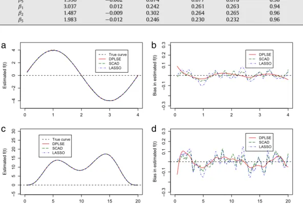
Fig. 5.1. Plots ofbf(t)and pointwise biases (SCAD and LASSO are based on converged MC samples). Plots (a) and (b) are forf1; plots (c) and (d) are forf2.

Heren=200 andσ2_{=1. The horizontal axis istin all the four plots.}

We report the results in four scenarios with varyingn,

σ

2_andf

₍

_t

₎

_{, and those in other scenarios are similar and hence} omitted. We observe that

b

β

is roughly unbiased in all scenarios. Both Bayesian and frequentist SEs of

b

β

_j’s obtained from(4.1) and(4.3)agree well with the empirical SEs; all SEs decrease asnincreases or

σ

2_{decreases. Bayesian SEs are slightly larger} than their frequentist counterparts, since they also account for bias in

b

β

_j. The confidence intervals based on either Bayesian or frequentist SEs achieve the nominal coverage probability, indicating the accuracy of the SE formulas. Overall, the DPLSE works very well for estimating model parameters.

5.3. Performance of

b

f

(

t

)

and pointwise standard errors

InFig. 5.1we plot the pointwise estimates and biases for estimatingf1

(

t

)

andf2

(

t

)

whenn

=

200 and

σ

2

=

1 for all three methods.

In plots (a) and (c), the averaged fitted curves are almost indistinguishable from the true nonparametric function, indicating small biases in

b

f

(

t

)

for all three methods. Pointwise biases are magnified in plots (b) and (d), which show that the DPLSE overall has smaller bias than the other two methods. The SCAD and LASSO fits have slightly larger and rougher pointwise biases, which indicate under-smoothing due to a small bandwidth selected by the plug-in method. Our method is more advantageous in that it automatically estimates the smoothing parameter and controls the amount of smoothing more appropriately by treating

τ

=

1

/(

n

λ

1

)

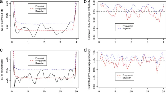
as a variance component.

Fig. 5.2depicts the pointwise standard errors and pointwise coverage probabilities of confidence intervals given by the covariance formulas(4.2)and(4.4). Heren

=

200 and

σ

2

₌

_{1; (a) and (b) are forf}

1witht6errors, and (c) and (d) are forf2 with mixture normal errors.

a

b

c

d

Fig. 5.2. Plots of pointwise frequentist and Bayesian standard errors and coverage probability rates. Plots (a) and (b) are forf1(t); plots (c) and (d) are for

f2(t). The horizontal axis istin all plots. Table 6.1

Estimated coefficients and frequentist and Bayesian SE for ragweed pollen level data.

Full model Selected model

Variable Parameter estimate Frequentist SE Bayesian SE Parameter estimate Frequentist SE Bayesian SE

x1 0.64 0.22 0.23 0.70 0.18 0.18 x2 1.31 0.37 0.39 1.16 0.36 0.37 x3 0.87 0.19 0.20 0.76 0.19 0.20 x2 2 0.53 0.23 0.24 0 – – x2 3 0.04 0.19 0.19 0 – – x1x2 0.26 0.19 0.19 0 – – x1x3 0.02 0.22 0.23 0 – – x2x3 0.34 0.20 0.20 0 – –

We note that the frequentist pointwise SEs interlace with the empirical SEs, whereas the Bayesian pointwise SEs are a little larger than the frequentist counterparts. Accordingly, as shown in plots (b) and (d), the pointwise coverage probability rates for frequentist confidence intervals are around the nominal level, whereas most of the Bayesian coverage probabilities are higher than 95%.

6. Real data application

We apply the proposed DPLS method to theRagweed Pollen Leveldata, which was analyzed in [8]. The data was collected in Kalamazoo, Michigan during the 1993 ragweed season, and it consists of 87 daily observations of ragweed pollen level and relevant information. The main interest is to develop accurate models to forecast daily ragweed pollen level. The raw responserag

w

eedis the daily ragweed pollen level (grains

/

m3_{). Among the explanatory variables,x}

1 is an indicator of significant rain, wherex1

=

1 if there is at least 3 h steady or brief but intense rain andx1

=

0 otherwise;x2is temperature (oF);x3is wind speed (knots). Thex-covariates are standardized first. Since the raw response is rather skewed, Ruppert et al. [8] suggested a square root transformationy

=

√

rag

w

eed. Marginal plots suggest a strong nonlinear relationship betweenyand the day number in the current ragweed pollen season. Consequently, a semiparametric regression model with a nonparametric baselinef

(

day

)

is reasonable. Ruppert et al. [8] fitted a semiparametric model withx1,x2andx3, whereas we add quadratic and interaction terms and consider a more complex model:

y

=

f

(

day

)

+

β

₁x1

+

β

2x2

+

β

3x3

+

β

22x22

+

β

33x23

+

β

12x1x2

+

β

13x1x3

+

β

23x2x3

+

ε.

The tuning parameter selected by BIC is

λ

2

=

0

.

177.Table 6.1gives the DPLSE for the regression coefficients and their corresponding frequentist and Bayesian standard errors.

For comparison, we also fitted the full model via traditional partially splines with only roughness penalty onf.Table 6.1 shows that the final fitted model is

b

y

=

b

f

(

day

)

+

b

β

1x1

+

b

β

2x2

+

b

β

3x3

,

indicating that the linear main effect model suffices.

day Estimated f(day) 95% Freq. C.I. Estimated f(day) 95% Bayesian C.I. 0 20 40 60 80 10 15 5 0

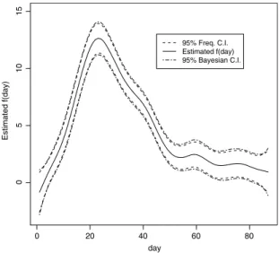
Fig. 6.1. Plot of estimatedf(day)and its frequentist and Bayesian 95% pointwise confidence intervals for the Ragweed Pollen Level data. All the estimated coefficients are positive, suggesting that the ragweed pollen level increases as each of the covariates increases. The shrinkage estimates have relatively smaller standard errors than those under the full model.Fig. 6.1depicts the estimated nonparametric function

b

f

(

day

)

and its frequentist and Bayesian 95% pointwise confidence intervals. The plot indicates that the baselinef

(

day

)

climbs rapidly to the peak on around day 25 and plunges until day 60, and decreases steadily thereafter.

7. Discussion

We propose a new regularization method for simultaneous variable selection and model estimation in partially linear models via double-penalized least squares. Under certain regularity conditions, the DPLSE

b

β

is root-nconsistent and has the oracle property. To facilitate computation, we reformulate the problem into a linear mixed model (LMM) framework, which allows us to estimate the smoothing parameter

λ

1as an additional variance component instead of conducting the conventional two-dimensional grid search together with the other tuning parameter

λ

2. Another advantage of the LMM representation is that standard software can be used to implement the DPLS. Simulation studies show that the new method works effectively in terms of both variable selection and model estimation. We have derived both frequentist and Bayesian covariance formulas for the DPLSEs and empirical results favor the frequentist SE formulas forf

(

t

)

. Furthermore, our empirical results suggest that the DPLSE is robust to the distributional assumption of errors, giving strong support for its application in general situations.

In this paper, we have studied the large-sample properties of the new estimators when the dimensiondsatisfies: (i)d

fixed, or (ii)dn

→ ∞

asn

→ ∞

withdn

<

n. In future research we will investigate the properties and performance of our

estimators for the more challenging situationd

n. Our major challenges will be to study how the convergence rate and asymptotic distributions of the linear components, in the presence of nuisance nonparametric components, will be affected whend

>

n. Very recently, Ravikumar et al. [35] and Meier et al. [36] consider the sparse estimation and function smoothing for additive models in high-dimensional data settings. We will see how these works can be adapted to tackle our challenges in the future.

The proposed DPLS method assumes that the errors are uncorrelated. In future research, we will generalize it to model selection for correlated data such as longitudinal data. Another interesting problem is model selection for generalized semiparametric models, e.g.E

(

Y

)

=

g

{

X

β

+

f

(

t

)

}

, whereg is a link function. In that case we will consider the double-penalized likelihood and investigate asymptotic properties for the resulting estimators.

Acknowledgements

The research of Hao Zhang was supported by in part by National Science Foundation DMS-0645293 and by National Institute of Health R01 CA085848-08. The research of Daowen Zhang was supported by National Institute of Health R01 CA85848-08.

Appendix. Proofs

Proof of Lemma 1.DifferentiatingL

(

β

)

inQ

(

β

)

and evaluating at

β

₀, we get:

L00

(

β

₀

)

=

XT

{

I

−

A

(λ

1

)

}

X

.

(A.2) For the partially linear model, we haveY

−

X

β

₀

=

f

+

ε

. Substitution into(A.1)yields

−

n−1/2L0

(

β

₀

)

=

n−1/2XT

{

I

−

A

(λ

1

)

}

(

f

+

ε

)

=

n−1/2XT

{

I

−

A

(λ

₁

)

}

f

+

ε

−

n−1/2XTA

(λ

₁

)

ε

.

(A.3)

Now, the proof of Theorem 1 in [4] and its four propositions can be used. Under regularity conditions, we have that if

λ

1n

→

0

andn

λ

1₁/_n4

→ ∞

, then n−1/2XT

{

I

−

A

(λ

1

)

}

f

+

ε

d

→

N

(

0

, σ

2R

),

(A.4) n−1/2XT_A

_(λ

1

)

ε

p

→

0

.

(A.5)

Parts (a) and (b) are obtained by applying Slutsky’s theorem to(A.1)and(A.2).

To proveTheorems 3and4, we need the following lemma. Its proof can be derived in the similar fashion asLemma 1 above and Theorem 1 of [4]. To save space, we only state the results below and omit the proof. For any vectorv, we use

[

v

]

_i to denote itsith component. For any matrixG, we use

[

G

]

_ijto denote its

(

i

,

j

)

th element.

Lemma 3. Under the regularity conditions

(

C1

)

and

(

C2

)

, if

λ

1n

→

0, then

(a)

L0

₍

_β

n0

)

i

=

Op

(

n 1/2

₎

_, (b)

L00

₍

_β

n0

)

ij

=

nRij

+

Op

(

n 1/2

_∨

_λ

−1/4 1n

)

.

Proof of Theorem 3. Letcn

=

√

dn

/

n. We need to show that for any given

>

0, there exists a large constantCsuch that

P

inf krk≥CQ

(

β

n0

+

cnr

) >

Q

(

β

n0

)

≥

1

−

.

(A.6)

Let∆n

(

r

)

=

Q

(

β

n0

+

cnr

)

−

Q

(

β

0

)

. Recall that the firstqncomponents of

β

n0are nonzero,pλ2n

(

0

)

=

0 andpλ2n

(

·

)

is

nonnegative. By the Taylor expansion, we have

∆n

(

r

)

≥

L

(

β

n0

+

cnr

)

−

L

(

β

n0

)

+

n qn

X

j=1

{

p_λ2n

(

|

β

_n10,j

+

cnrj

|

)

−

pλ2n

(

|

β

n10,j

|

)

}

≥

cnrTL0

(

β

n0

)

+

1 2c 2 nr T_L00

₍

_β

n0

)

r

+

qn

X

j=1

[

ncnp0_λ2n

(

|

β

n10,j

|

)

sign

(β

n10,j

)

rj

] +

qn

X

j=1

[

nc_n2p00_λ2n

(

|

β

_n10,j

|

)

r_j2

{

1

+

o

(

1

)

}]

≡

I1

+

I2

+

I3

+

I4

.

ByLemma 3(a), we have

|

I1

| = |

cnrTL0

(

β

n0

)

| ≤

cn

k

L0

(

β

n0

)

k k

r

k =

Op

(

cn

p

ndn

)

k

r

k =

Op

(

ncn2

)

k

r

k

.

ByLemma 3(b), under the regularity condition (C2), we have

I2

=

1 2c 2 nr T_L00

₍

_β

n0

)

r

=

1 2nc 2 n

{

r T_Rr

₊

_O p

(

dnn−1/2

∨

dn

λ

−1/4 1n

)

}

=

1 2nc 2 n

{

r T_Rr

₊

_o p

(

1

)

k

r

k

2

}

,

the last equation above is due to the dimension conditiondn

=

o

(

n1/2

∧

n

λ

11/n4

)

. With regard toI3andI4, we have

|

I3

| ≤

qn

X

j=1

|

ncnp0_λ2n

(

|

β

n10,j

|

)

sign

(β

n10,j

)

rj

| ≤

ncn2

k

r

k

,

and

|

I4

| =

qn

X

j=1 nc2_np00_λ2n

(

|

β

_n10,j

|

)

r_j2

{

1

+

o

(

1

)

} ≤

2

·

max 1≤j≤qn p00_λ2n

(

|

β

_n10,j

|

)

·

nc_n2

k

r

k

2

.

Under the condition (C1), max1≤j≤qnp

0

λ2n

(

|

β

n10,j

|

)

=

0 and max1≤j≤qnp 00

λ2n

(

|

β

n10,j

|

)

=

0 whennis large enough and

λ

2n

→

0.

So, bothI3andI4are dominated byI2. Therefore, by allowingCto be large enough, all termsI1

,

I3

,

I4are dominated byI2, which is positive. This proves(A.6)and completes the proof.