Estimation of generalized linear latent variable models via fully exponential Laplace approximation

(1)

Contents lists available atSciVerse ScienceDirect

Journal of Multivariate Analysis

journal homepage:www.elsevier.com/locate/jmva

Estimation of generalized linear latent variable models via fully

exponential Laplace approximation

Silvia Bianconcini, Silvia Cagnone

∗

Department of Statistics, University of Bologna, Italy

a r t i c l e i n f o Article history:

Received 29 August 2011 Available online 1 July 2012 AMS subject classifications: 62H12 62F12 Keywords: Laplace approximation Adaptive Gauss–Hermite EM algorithm Ordinal data

a b s t r a c t

Latent variable models represent a useful tool in different fields of research in which the constructs of interest are not directly observable. In such models, problems related to the integration of the likelihood function can arise since analytical solutions do not exist. Numerical approximations, like the widely used Gauss–Hermite (GH) quadrature, are generally applied to solve these problems. However, GH becomes unfeasible as the number of latent variables increases. Thus, alternative solutions have to be found. In this paper, we propose an extended version of the Laplace method for approximating the integrals, known as fully exponential Laplace approximation. It is computational feasible also in presence of many latent variables, and it is more accurate than the classical Laplace approximation. The method is developed within the Generalized Linear Latent Variable Models (GLLVM) framework.

1. Introduction

Latent variable models represent a useful tool in the social sciences where the analyzed constructs cannot be directly observed and, hence, they are not measurable. However, a set of indicators related to each unobserved variable can be measured. These models can be defined within the Generalized Linear Latent Variable Model (GLLVM) framework [2,16], according to which the entire set of the responses given by an individual to a certain number of items, called the response pattern, is expressed as a function of one or more latent variables through a monotone differentiable link function. The estimation of the model parameters can be obtained by means of a full information maximum likelihood method via the EM algorithm, that guarantees quite accurate estimates [14,15].

The presence of the latent variables causes problems related to the integration of the likelihood function when the observed variables are discrete, since analytical solutions do not exist. In order to overcome this drawback, numerical approximations are usually applied. One of the most often used techniques is the classical Gauss–Hermite (GH) quadrature [3], that provides quite good parameter estimates when many quadrature points are considered per each latent variable. However, it becomes computationally unfeasible as the number of latent variables increases. This represents a serious limitation for a large number of applications where several observed and latent variables are required [5].

As alternative solution to GH, the Adaptive Gauss–Hermite (AGH) quadrature has been discussed for different models with random effects and/or latent variables [17,19,23]. In all these studies, AGH is shown to perform better than GH, also when few quadrature points are used. Indeed, it consists of adjusting the GH nodes with the first and second moments of the posterior density of the latent factors given the manifest variables. This allows a better approximation of the function to be integrated. Nevertheless, the AGH is very computationally intensive, particularly when the observed variables have many categories [4].

∗_{Corresponding author.}

E-mail address:[email protected](S. Cagnone).

(2)

An approximation technique that is not affected by the presence of high dimensional integrals is the Laplace method [7,1], that can be viewed as a particular case of the AGH when just one abscissa is used [11]. Given its reduced dimensionality, the Laplace method is one of the fastest techniques, since the computational burden depends only on the calculation of the mode of the integrand [25,20,8,18]. It has been used to estimate GLLVM by [8]. These authors showed that when this approximation is applied to maximize the likelihood function of a general GLLVM using a Newton–Raphson scheme, the asymptotic error is of orderO

(

p−1

₎

_{, with}_p_{number of items, and hence it is not directly controllable. Joe} [9] has investigated the performance of the Laplace technique for a variety of discrete response mixed models, and he has found that it becomes less adequate as the degree of discreteness increases. A way to overcome these limitations is to consider higher order Laplace approximations as proposed by [20]. However, this extension is quite unfeasible in practice, in particular for GLLVM, since it involves combinations of higher (than two) order derivatives of the likelihood function. Recently, [22] developed the Integrated Nested Laplace Approximation (INLA) to perform Bayesian inference of latent Gaussian models with non-Gaussian observations. This procedure combines Laplace approximations with numerical integration to provide a fast and accurate method for approximating the predictive density of the latent variables/random effects. The approach finds a direct application in generalized linear mixed models, and its main computational advantages are in effect when the inverse covariance matrix of the random effects is sparse and the number of parameters is small.

When either the EM algorithm or a direct maximization of the observed data log-likelihood is used for model estimation, an extended version of the Laplace method, called Fully exponential Laplace Approximation (FLA), can be applied. It has been introduced and developed by [26] in the Bayesian context for approximating posterior distributions. Recently, it has been extended by [21] to a variety of models for longitudinal continuous measurements and time-to-event data estimated via the EM algorithm. The main idea proposed by these authors is to apply the FLA to the expected score function of the model parameters with respect to the posterior distribution of the latent variables. With the FLA, a better approximation of the multidimensional integrals is achieved, being the approximation error of orderO

(

p−2

)

. Moreover, the computational complexity of this approach is similar to the classical Laplace method since it depends only on the numerical optimization required to compute the mode of the integrand. In this paper, we extend the FLA to the general class of the GLLVM. In detail, in Section2the GLLVM is introduced, in Section3the estimation problem is discussed considering the FLA. In Section4, a simulation study for the particular case of ordinal data is performed in order to compare the finite sample and asymptotic properties of the AGH, classical Laplace and FLA under different conditions. Finally, Section5gives the conclusions.

2. Model specification

Lety

=

(

y1

, . . . ,

yp

)

be a vector ofpobserved variables of any type andz

=

(

z1

, . . . ,

zq

)

be a vector ofqlatent variables.

The distributionf

(

y

)

of the manifest variables can be expressed as f

(

y

)

=



Rq

g

(

y

|

z

)

h

(

z

)

dz

,

(1)

whereh

(

z

)

is the density function ofzand it is assumed to be normal with null mean and correlation matrix equal to9, and g

(

y

|

z

)

is the conditional density function ofygivenz. Under the assumption of conditional independence ofygivenz, the association among the observed variables is assumed to be wholly explained by the latent variables, so that

g

(

y

|

z

)

=

p



i=1

gi

(

yi

|

z

).

(2)

According to the GLLVM framework, each conditional distribution gi

(

yi

|

z

)

belongs to the exponential family and

constitutes the random component of the generalized model. More specifically, gi

(

yi

|

z

)

=

exp



yi

θ

i

(

z

)

−

bi

(θ

i

(

z

))

φ

i

+

ci

(

yi

, φ

i

)



,

(3)

where

θ

i

(

z

)

is the canonical parameter;bi

(θ

i

(

z

))

andci

(

yi

, φ

i

)

are specific functions that assume different forms according

to the different nature ofyi;

φ

iis a scale parameter. In particular,

b′_i

(θ

i

(

z

))

=

E

(

yi

|

z

)

=

µ

i

(

z

).

The systematic component of the model is given by

η

i

=

τ

i

+

q



j=1

α

ijzj

,

(4)

where

τ

i is the intercept and

α

ij can be interpreted as factor loadings of the model. The link between the systematic

component and the conditional mean of the random component is

η

i

=

ν

i

[

µ

i

(

z

)

]

, where

ν

i can be any monotonic,

(3)

In the following, we give the specification of GLLVM for responses characterized by different degrees of discreteness, for which the integration problem arises. That is,

•

binary data:

gi

(

yi

|

z

)

follows a Bernoulli distribution

gi

(

yi

|

z

)

=

π

iyi

(

1

−

π

i

)

1−yi (5)

that can be also written in the exponential form as gi

(

yi

|

z

)

=

exp



yilog



π

i 1

−

π

_i



+

log

(

1

−

π

_i

)



(6) with

π

i

=

exp



τ

i

+

q



j=1

α

ijzj



1

+

exp



τ

i

+

q



j=1

α

ijzj



,

θ

i

(

z

)

=

logit

(π

i

),

bi

(θ

i

(

z

))

=

log

(

1

+

exp

(θ

i

(

z

))),

φ

i

=

1

,

ci

(

yi

, φ

i

)

=

0

;

•

count data:

gi

(

yi

|

z

)

follows a Poisson distribution

gi

(

yi

|

z

)

=

µ

i

(

z

)

yi

!

exp

(

−

µ

_i

(

z

))

(7)

that can be also written as

gi

(

yi

|

z

)

=

exp [yilog

µ

i

(

z

)

−

µ

i

(

z

)

−

ln

(

yi

!

)

] (8) with

θ

i

(

z

)

=

ln

µ

i

(

z

)

=

τ

i

+

q



j=1

α

ijzj bi

(θ

i

(

z

))

=

exp

(θ

i

(

z

))

=

µ

i

(

z

),

φ

i

=

1

,

ci

(

yi

, φ

i

)

= −

ln

(

yi

!

)

;

•

ordinal data:

gi

(

yi

|

z

)

follows a multinomial distribution

g_i

(

y_i

|

z

)

=

ci



s=1

(γ

i,s

(

z

)

−

γ

i,s−1

(

z

))

yi,s

,

(9) withcinumber of categories for the itemyi,yi,s

=

1 if the response is in categorysand 0 otherwise,

γ

i,s

(

z

)

=

P

(

yi

≤

s

|

z

)

s

=

1

, . . . ,

cidefined as

γ

i,s

(

z

)

=

exp



τ

i

−

q



j=1

α

ijzj



1

+

exp



τ

i

−

q



j=1

α

ijzj



.

In this case,

τ

i,sare category-specific intercepts such that

τ

i,1

≤

τ

i,2

≤ · · · ≤

τ

i,s

= +∞

. The negative sign in front of the

loadings indicates that the probability to fall in high categories ofyiincreases aszincreases.

To complete the specification of the model, denoting for simplicity

γ

_i_,_s

=

γ

_i_,_s

(

z

)

, we can rewriteg_i

(

y_i

|

z

)

in the exponential form as follows

gi

(

yi

|

z

)

=

exp



_c i−1



s=1



y∗_i_,_slog

γ

i,s

γ

i,s+1

−

γ

i,s

−

y∗_i_,_s₊₁log

γ

i,s+1

γ

i,s+1

−

γ

i,s





,

(10)

wherey∗_i_,_s

=

1 if the response is in categorysor lower ofith variable and 0 otherwise,

θ

i,s

(

z

)

=

log

γ

i,s

γ

i,s+1

−

γ

i,s

,

bi

(θ

i,s

(

z

))

=

log

(

1

+

exp

(θ

i,s

(

z

))),

(4)

3. Model estimation

Model estimation is achieved by using the maximum likelihood through the EM algorithm, since the latent variables are unknown. At this regard, we apply a full information maximum likelihood method by which all the parameters of the model are estimated simultaneously. For the sake of simplicity, in the following we consider9

=

I.

For a random sample of sizen, from Eq.(1), the observed data log-likelihood is defined as L

=

n



l=1 logf

(

y_l

)

=

n



l=1 log



Rq g

(

y_l

|

z_l

)

h

(

z_l

)

dz_l

.

(11)

The EM algorithm consists of an Expectation step (E-step), in which the expected score functionE

(

S

(

a_i

))

of the model parametersa′

i

=

(τ

i

, α

i1

, . . . , α

iq

),

i

=

1

, . . . ,

p, is computed. The expectation is with respect to the posterior distribution

h

(

zl

|

yl

)

ofzgiven the observations for each individual. In the Maximization step (M-step), updated parameter estimates

are obtained by equating to 0 the expected score functions.

Louis [12] proved that the observed data score vector

∂

L

/∂

aiis equivalent to the expected score functionE

(

S

(

ai

))

with

respect toh

(

zl

|

yl

)

, so that

∂

L

∂

ai

=

E

(

S

(

ai

))

=

n



l=1



S

(

ai

)

g

(

yl

|

zl

)

h

(

zl

)

dzl



g

(

yl

|

zl

)

h

(

zl

)

dzl

=

n



l=1



∂

logg

(

yl

|

zl

)

∂

ai h

(

zl

|

yl

)

dzl i

=

1

, . . . ,

p (12)

From Eq.(12), it can be noticed that the computation of the expected score functions involves a multidimensional integral that cannot be solved analytically, hence numerical approximations are required. In particular, in the following, we propose the use of the extended version of the classical Laplace approximation, that is the fully exponential Laplace method. 3.1. Fully exponential Laplace approximation method

The FLA method has been proposed for the first time by [26] in order to approximate posterior distributions in the Bayesian context. It represents an extension of the classical Laplace approximation that, as is known, is based on the second order Taylor expansion of the logarithm of the integrand, with the latent variables evaluated at the mode (see, among the others, [25]).

The Laplace method has the advantage of dealing with integrals of any dimensionality without introducing computational problems but, for the general class of latent variable models discussed in this paper, it produces an approximation error of orderO

(

p−1

)

, that can be reduced only increasing the number of observed variables. The FLA leads to an improvement of the approximation error maintaining the same computational complexity as the classical Laplace method. The extension of FLA to joint models for continuous longitudinal measurements and time-to-event data has been proposed by [21]. It requires the computation of the following quantities

E

(

A

(

zl

))

=



A

(

zl

)

h

(

zl

|

yl

)

dzl

=



A

(

z_l

)

g

(

y_l

|

z_l

)

h

(

z_l

)

dz_l



g

(

yl

|

zl

)

h

(

zl

)

dzl (13) that differ from(12)sinceA

(

· )

are the components of the score functionsS

(

ai

)

that depend on the latent variables.

The main idea of FLA is to approximate both the numerator and the denominator in Eq.(13)with the classical Laplace method. Tierney and Kadane [25] proved that the error terms of orderO

(

p−1

)

in the numerator and the denominator cancel out, leading to a smaller error term of orderO

(

p−2

₎

_{. The development of FLA is strictly related to the form of the score} function, which strongly depends on the type of data, that is on the associated member of the exponential family. For the specific cases discussed above we obtain

•

Binary data A1,i

(

zl

)

= −

∂

bi

(θ

i

(

zl

))

∂τ

i

= −

π

_i

(

zl

)

A2,i

(

zl

)

=

∂

loggi

(

yi,l

|

zl

)

∂α

i

=

zl

(

yi

−

π

i

(

zl

)).

•

Count data A1,i

(

zl

)

= −

∂

bi

(θ

i

(

zl

))

∂τ

i

= −

µ

_i

(

z_l

)

A2,i

(

zl

)

=

∂

loggi

(

yi,l

|

zl

)

∂α

i

=

zl

(

yi

−

µ

i

(

zl

)).

(5)

•

Ordinal data A1,i,s

(

zl

)

= −

∂θ

i,s−1,l

(

zl

)

∂τ

i,s

=



(

₁

₋

γ

i,s,l

),

ifs

=

1

;

(

1

−

γ

_i_,_s_,_l

)

γ

i,s,l

(γ

i,s,l

−

γ

i,s−1,l

)

,

ifs

=

2

, . . . ,

ci

−

1

.

A2,i,s

(

zl

)

=

∂

bi

(θ

i,s,l

(

zl

))

∂τ

i,s

=

(

1

−

γ

_i_,_s_,_l

)

γ

i,s,l

(γ

i,s+1,l

−

γ

i,s,l

)

s

=

1

, . . . ,

ci

−

1

.

A3,i,s

(

zl

)

= −

∂

loggi

(

yi,s,l

|

zl

)

∂α

i

=



(

1

−

γ

_i_,_s_,_l

)

zl

,

ifs

=

1

;

(

1

−

γ

_i_,_s_,_l

−

γ

_i_,_s₋₁_,_l

)

zl

,

ifs

=

2

, . . . ,

ci

.

The FLA approximation can be applied only to strictly positive functionsA

(

· )

. In our case, this condition is not necessarily guaranteed since theA

(

· )

are components of the score functions, not constrained to be positive. To overcome this problem, the method of the moment generating function can be used. According to this approach, since the quantity exp

{

t′_A

₍

_z

l

)

}

is always positive, the FLA approximation can be applied to the moment generating functionM

(

t

)

=

E

[

exp

{

t′_A

₍

_z

l

))

}

,

with latent variableszlevaluated at the mode

ˆ

zl

=

arg maxzl

[

logg

(

yl

|

zl

)

+

logh

(

zl

)

+

t

′

A

(

zl

)

]

. In doing so, we get the

approximated moment generating functionM

ˆ

(

t

)

. Hence, from the corresponding cumulant-generating function logM

ˆ

(

t

)

, we obtain the approximated expected valuesE

ˆ

(

A

(

zl

))

. These latter values are the quantities of interest, and they are given

by

ˆ

E

(

A

(

zl

))

=

∂

t log

ˆ

M

(

t

)



t=0

=

∂

tlog

ˆ

E

[

exp

{

t′A

(

zl

)

}]



t=0

.

(14) Tierney et al. [26] proved (Theorem 2, p. 712) that Eq.(14)is equivalent to the following expression

ˆ

E

(

A

(

z_l

))

=

A

(

z

ˆ

_l

)

+

∂

log det

(

6 (t) l

)

−1/2

∂

t



₍ zl=ˆzl,t=0)

+

O

(

p−2

)

=

A

(

z

ˆ

l

)

−

1 2tr

(

)



₍ zl=ˆzl,t=0)

+

O

(

p−2

),

(15) where 6(t) l

= −

∂

2

_{

_log_g

₍

_y l

|

zl

)

+

logh

(

zl

)

+

t′A

(

zl

)

}

∂

z′_l

∂

zl (16) and

=

6−1_l

{

∂

6(_lt)

/∂

t

}

.

The expressions of the first derivatives of6lwith respect totare reported in theAppendix.

3.2. EM algorithm

The steps of the EM algorithm are defined as follows:

1. Choose initial values for the parameters of the model and for the mode.

2. Compute the mode

ˆ

zl

,

l

=

1

, . . . ,

n, by using a Newton–Raphson iterative scheme. In more detail, for the

(

m

)

-th iteration

ˆ

z_lm

= ˆ

z(_lm−1)

− [

(

6_l(m−1)

)

−1S

(

z(_lm−1)

)

]|

(zl=ˆz(lm−1),t=0)

,

where6lis the Hessian matrix defined in expression(16)andS

(

zl

)

is defined as follows

S

(

zl

)

= −

∂

{

logg

(

yl

|

zl

)

+

logh

(

zl

)

+

t′A

(

zl

)

}

∂

zl

.

(17) 3. E-step. Compute the FLA expected valuesE

ˆ

(

A

(

zl

))

, and the approximated expected score functionE

ˆ

(

S

(

ai

))

, where

i

=

1

, . . . ,

p.

4. M-step. Obtain improved estimates for the model parameters. For all of them, a Newton–Raphson iterative scheme is used in order to solve the corresponding nonlinear maximum likelihood equations.

5. Repeat steps 2–4 until convergence is attained.

In the following section, we perform a simulation study for the model with ordinal variables reported in expression(9). The choice of this particular model has been mainly motivated by three reasons. The first one is that ordinal data are very diffused in analysis carried out in the social sciences. The second one is that latent variable models with ordinal data are the most affected by computational burden due to integration problems. Finally, the FLA method for the model with ordinal variables is the most complex to derive among the cases discussed in Section2. All the technical details for the application of FLA in presence of ordinal data are reported in theAppendix.

(6)

Table 1

Mean, bias and MSE of the parameter estimates for AGHme, and AGHmo, Lap, and FLA in the generated data.

AGH Lap FLA

Mean Mode

% Valid samples 82 72 66 70

True Mean Bias MSE Mean Bias MSE Mean Bias MSE Mean Bias MSE

α11=1.03 1.37 0.34 0.63 1.47 0.44 0.61 1.17 0.14 0.21 1.02 −0.01 0.03 α21=1.44 1.41 −0.02 0.41 1.26 −0.18 0.34 0.82 −0.61 0.62 1.62 0.18 0.17 α31=2.11 2.22 0.10 0.68 1.96 −0.15 0.37 1.21 −0.90 1.04 2.31 0.20 0.33 α41=1.80 1.91 0.11 0.61 1.75 −0.05 0.43 1.21 −0.59 0.56 1.52 −0.28 0.15 α51=1.53 1.58 0.05 0.40 1.42 −0.10 0.25 1.23 −0.30 0.30 1.80 0.27 0.26 α12=0.00 – – – – – – – – – – – – α22=2.42 1.99 −0.42 0.74 2.09 0.33 0.46 1.85 −0.57 0.57 2.01 −0.41 0.36 α32=1.52 1.70 0.18 0.51 1.80 0.27 0.44 1.38 −0.14 0.24 1.98 0.46 0.44 α42=0.75 0.76 0.01 0.49 0.93 0.18 0.35 1.37 0.62 0.56 1.01 0.26 0.12 α52=1.34 1.50 0.16 0.44 1.43 0.26 0.41 1.96 0.62 0.39 1.70 0.36 0.31 4. Simulation study

The properties of the FLA method in the GLLVM for ordinal data can be evaluated by performing a simulation study in which several conditions are taken into account. The results will be compared with those obtained with the classical Laplace (Lap) as applied by [8,9], and with the AGH quadrature. In recent years, the latter has been widely applied in latent variable models, since it allows to obtain estimates that are as accurate as those derived by the GH technique, but using a smaller number of quadrature points. It essentially consists of scaling and translating the classical Gaussian quadrature locations to place them under the peak of the integrand, and two different procedures have been adopted in the literature. According to the first one, the mode of the integrand and the inverse of the information matrix of the integrand evaluated at the mode are computed [11,17,23]. The advantage of this approach lies in the fact that the quadrature points are not involved in these computations. However, this method is computationally demanding since it requires numerical optimization routines and the computation of second derivatives. Moreover, when parameter estimates are obtained by using iterative algorithms, like in our case, the first and second order moments have to be computed at each step, hence the algorithm becomes very slow. An alternative procedure consists of computing the posterior means and covariance matrices at each step of the algorithm [19]. Although this method requires the use of quadrature points themselves, the posterior moments should better describe the integrand in those cases in which its tails are heavier than the normal density. In the following, we show how both these techniques work in latent variable models for ordinal data, and we compare their performances with FLA.

The software used for the analyses are Fortran 95 and R. The codes are available from the authors upon request. 4.1. Finite sample properties of the estimators

To investigate empirically the finite sample performance of the FLA, Lap and AGH, based on both the posterior mean

(

AGHme

)

and mode

(

AGHmo

)

, we generated data from a population that consists of five variables and satisfies a two factor

model. The number of categories is the same for each observed variable, and equal to 4. 500 random samples were considered withn

=

200 subjects. We chose 5 quadrature points per each latent variable for both the adaptive approximations. We also considered 7 quadrature points, but there was a little difference with 5 nodes, suggesting that the latter provides sufficient accuracy for this example.

The population parameters were chosen in such a way that the thresholds range from

−

3 to 3. The factor loadings are the following:

α

1

=

(

1

.

03

,

1

.

44

,

2

.

11

,

1

.

8

,

1

.

53

)

and

α

2

=

(

0

,

2

.

42

,

1

.

52

,

0

.

75

,

1

.

34

)

with not null values generated from a log-normal distribution, and one loading fixed to 0 to get a unique solution.

Table 1reports the mean, bias, and Mean Square Error (MSE) of the parameter estimates obtained by applying all the techniques. The results show that the percentage of valid samples is quite high for all the procedures apart from Lap, ranging from 66% to 82%. The FLA presents much better MSE values than those achieved by Lap, AGHmeand AGHmo. The superior

performance of FLA compared with Lap is mainly due to the larger bias that characterizes the values obtained with the classical method. This is in agreement with the findings given by [9] in the case of ordinal data. Furthermore, FLA performs better than the quadrature techniques mainly because of a smaller variability of the estimates. Comparing the adaptive techniques, AGHmeestimates are less biased than those determined by AGHmo, and present an opposite sign of the bias

for several values of

α

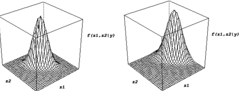
1. On the other hand, the latter behaves better in terms of MSE values. The different performance of the two adaptive techniques can be due to the fact that the individual posterior densities to be approximated are not always symmetric. In latent variable models for ordinal data, [6] proved that the posterior densities asymptotically follow a multivariate normal distribution. However, for a small number of observed variables, the integrand could be skewed, and the numerical procedures could provide quite different results.

To analyze the shape of the individual posterior densities in the generated population, we computed measures of multivariate skewness

β

1,qand kurtosis

β

2,qproposed by Mardia (1970). In the case of two latent variables, they are given

(7)

Fig. 1. Individual posterior densities with different shapes (on the left sideβ1,2=0.000, and on the right sideβ1,2=0.168) in the generated population of 200 subjects. by

β

1,2

(

l

)

=

µ

230

+

µ

2 03

+

3

µ

2 12

+

3

µ

2 21 l

=

1

, . . . ,

n and

β

2,2

(

l

)

=

µ

04

+

µ

40

+

2

µ

22 l

=

1

, . . . ,

n with

µ

ij

=

E

(

z1ilz j

2l

)

, whereasz1landz2lare the latent factors standardized with respect to the posterior densities. Mardia

(1970) also derived the asymptotic distributions of both

β

1,qand

β

2,q, and the corresponding statistical tests to evaluate the

null hypothesesH0

:

β

1,q

=

0 andH0

:

β

2,q

=

q

(

q

+

2

)

, beingq

(

q

+

2

)

the kurtosis inq-variate normal densities.

By computing these measures for the individual posterior densities generated in this simulation study, we observed that about 35% of these functions have a significant skewness, and a kurtosis always not significantly different from 8. In particular,

β

1,2is on average equal to 0.044 and it ranges from 0.000 to the significant value 0.168. The presence of individual posterior densities having different shapes could justify the different behavior of AGHs and FLA. InFig. 1, we show two different functions obtained from our generated data. In order to better analyze the finite sample properties of FLA and AGHs, we also generated data from two hypothetical extreme scenarios: one in which all the posterior densities are symmetric, and another one in which a high percentage (more than 60%) of the densities are skewed. As before, we consider five observed variables, each with 4 categories, satisfying a two factor model. The results for both the populations are shown inTable 2.

In the first scenario, the thresholds for each item are equal to

−

2 for the first category, 0 for the second, and 2 for the third one, whereas the loadings are all fixed to 0.5 except one set equal to zero. In this population, all the individual posterior densities are symmetric, with

β

1,2on average equal to 0.005, and

β

2,2always not significantly different from 8. As in the previous simulation study, we generated 500 random samples with 200 subjects.

For all the samples the algorithm achieves the convergence for FLA and AGHme, and in the 96% of the cases for AGHmo. The

FLA improves a lot with respect to the previous case, with a reduction of almost one digit in the MSE values, mainly due to smaller bias values for

α

2. On the other hand, both the AGH techniques provide better results in terms of bias and MSE, even if they still perform worse than FLA. We can also notice that the results provided by the two adaptive procedures are almost the same, with an equal sign of the bias for all the estimates, and slight discrepancies due to the different computational techniques involved. Indeed, as discussed by [19], the two procedures should provide similar results when the posterior densities are symmetric.

In the second scenario, the thresholds for each item are equal to

−

1 for the first category, 0 for the second, and 1 for the third one, whereas the loadings are fixed equal to

α

1

=

(

2

.

5

,

2

.

5

,

2

.

5

,

2

.

5

,

2

.

5

)

and

α

2

=

(

0

,

1

,

1

,

1

,

1

)

. In this case, 65% of the posterior densities are skewed.

β

1,2ranges from 0.000 to 0.239, the latter being significantly different from zero, and it is on average equal to 0.127. On the other hand, there is no significant kurtosis for all the subjects. The main consequence of this high percentage of skew densities is that, for both FLA and AGHmo, a very small number of samples (26% for the former,

18% for the latter) converge properly. Hence, the results are not reliable. On the other hand, AGHmeseems to be unaffected

by the different shapes of the posterior densities. Its results are more stable in terms of mean, bias, and MSE of the estimates as well as in terms of percentage of valid samples, that also in this case is 73%.

From these results, we can argue that FLA will be superior than AGH when the majority of the posterior densities is symmetric. In these cases, the former provides better MSE values for the estimates than the latter, mainly due to a reduced variability in the estimates. Moreover, the bias introduced in the estimates using FLA is quite comparable with the one in the AGH estimates. On the other hand, we have also shown that the AGHmeprovides more stable results, that are not

affected by the shape of the integrand. Its use is then suggested in populations characterized by a high percentage of skew distributions. It is interesting to highlight that, even if crucial when assessing simulations in such kind of studies, we cannot draw conclusions on the relation between the degree of dependence between items and the behavior of the FLA. Indeed, further investigations of the shape of the individual posterior densities have highlighted that their skewness

(8)

Table 2

Mean, bias and MSE for FLA, AGHme, and AGHmofor different scenarios in finite samples.

AGH FLA

Mean Mode

% Valid samples 90 100 100

True Mean Bias MSE Mean Bias MSE Mean Bias MSE

α11=0.5 0.90 0.40 0.69 0.84 0.34 0.61 0.59 0.09 0.02 α21=0.5 0.52 0.02 0.37 0.55 0.04 0.46 0.61 0.11 0.02 α31=0.5 0.47 −0.02 0.41 0.47 −0.03 0.47 0.60 0.10 0.02 α41=0.5 0.48 −0.02 0.42 0.55 0.05 0.60 0.60 0.10 0.02 α51=0.5 0.51 0.01 0.42 0.53 0.03 0.48 0.60 0.10 0.02 α12=0.0 – – – – – – – – – α22=0.5 0.73 0.23 0.57 0.72 0.22 0.65 0.60 0.10 0.01 α32=0.5 0.73 0.23 0.68 0.70 0.20 0.71 0.59 0.09 0.01 α42=0.5 0.65 0.15 0.54 0.63 0.13 0.67 0.59 0.09 0.01 α52=0.5 0.72 0.22 0.58 0.68 0.19 0.56 0.59 0.09 0.02 % Valid samples 73 18 26

True Mean Bias MSE Mean Bias MSE Mean Bias MSE

α11=2.5 2.47 −0.03 0.31 2.34 −0.16 0.25 2.97 0.47 0.86 α21=2.5 2.71 0.21 0.44 2.41 −0.08 0.14 2.28 −0.22 0.25 α31=2.5 2.73 0.23 0.48 2.44 −0.06 0.11 2.21 −0.29 0.22 α41=2.5 2.71 0.21 0.36 2.57 0.07 0.19 2.28 −0.22 0.20 α51=2.5 2.77 0.27 0.50 2.52 0.02 0.11 2.27 −0.23 0.29 α12=0.0 – – – – – – – – – α22=1.0 1.12 0.13 0.49 0.93 −0.07 0.38 1.92 0.92 0.93 α32=1.0 1.15 0.15 0.59 0.97 −0.03 0.33 1.84 0.84 0.80 α42=1.0 1.09 0.09 0.52 0.98 −0.02 0.34 1.91 0.91 0.89 α52=1.0 1.24 0.24 0.65 0.89 −0.11 0.45 1.97 0.97 0.98

also depends on the thresholds. As these latter increase, the skewness decreases for given values of the loadings. It means that scenarios characterized by high values of thresholds and quite high values of the loadings imply high and significant polychoric correlations between the observations and a high percentage of symmetric posterior densities. For example, using the loadings selected in the second scenario ofTable 2with thresholds ranging from

−

3 to 3 instead of ranging from

−

1 to 1, the percentage of asymmetric posterior densities decreases from more than 60% to almost 15%. In this case, differently from what is obtained for the second scenario, FLA performs very well. However, in both cases the polychoric correlations between items are in general quite high, indicating that there is no evidence of a direct relation between the FLA behavior and the degree of dependence between manifest variables.

4.2. Asymptotic properties of estimators

The asymptotic properties of the Laplace maximum likelihood estimators

θ

ˆ

have been derived and discussed by [21]. Under suitable regularity conditions, these authors showed that

ˆ

θ

−

θ

₀

=

Op



max



n−1/2

,

p−2



,

where

θ

0denotes the true parameter value.

θ

ˆ

will be consistent as long as bothnandpgrow to

∞

. FLA is superior than standard Laplace method, since the latter produces estimators with an approximation error of orderOp



max



n−1/2

_,

_p−1



. On the other hand, following [11,26], it can be shown that FLA shares the same approximation error of the AGH with 5 quadrature points.

To assess the asymptotic accuracy of the FLA estimator as well as of the classical Laplace, we generated 500 random samples with 1000 subjects from the population described in the previous section. We also applied both the adaptive techniques, and the results are shown inTable 3.

The percentage of valid samples is quite high for all the techniques, apart from Lap, ranging from 65% to 94%. FLA has a good performance as before with small MSE and bias values. On the other hand, both AGHs have an analogous behavior: the MSE values are drastically reduced with respect to the finite sample situation, and the bias is small for all the parameters.

It is worth noting that again FLA performs much better than the classical Laplace approximation, also in this case for the higher biases of the estimates obtained with the latter method. On the other hand, the bias in the AGH and FLA estimates is quite comparable, with a slightly better performance of the former for the second factor loadings (Table 3).

To better investigate the asymptotic properties of the FLA as function not only of the number of individualsn, but also of the number of itemsp, we performed a numerical study in which the performance of the FLA is compared with AGHmein

the presence of ten observed items, each of them characterized by four categories, assumed to satisfy a four factor model. We compared FLA only with AGHmesince the computational burden of this simulation is quite heavy and in the previous

study, forn

=

1000

,

AGHmeand AGHmogave very similar results, whereas Lap performed worse than all the other methods.

(9)

Table 3

Mean, bias and MSE for AGHme,AGHmo, Lap and FLA for generated data withn=1000.

AGH Lap FLA

Mean Mode

% Valid samples 92 94 65 90

True Mean Bias MSE Mean Bias MSE Mean Bias MSE Mean Bias MSE

α11=1.03 1.11 0.07 0.07 1.14 0.11 0.09 1.12 0.09 0.24 1.00 0.03 0.01 α21=1.44 1.41 −0.03 0.10 1.36 −0.07 0.10 0.78 −0.66 0.66 1.59 0.15 0.07 α31=2.11 2.08 −0.03 0.08 2.04 −0.07 0.09 1.17 −0.93 1.15 2.25 0.14 0.08 α41=1.80 1.82 0.02 0.11 1.79 0.01 0.13 1.08 −0.71 0.77 1.52 0.28 0.09 α51=1.53 1.52 −0.01 0.05 1.48 −0.05 0.06 1.19 −0.33 0.33 1.72 0.19 0.08 α12=0.00 – – – – – – – – – – α22=2.42 2.21 −0.21 0.18 2.24 −0.18 0.19 1.86 −0.56 0.53 2.00 −0.42 0.25 α32=1.52 1.58 0.06 0.11 1.64 0.12 0.12 1.31 −0.21 0.32 1.88 0.36 0.18 α42=0.75 0.74 −0.01 0.11 0.79 0.04 0.09 1.34 0.59 0.58 0.96 0.21 0.06 α52=1.34 1.40 0.06 0.07 1.44 0.10 0.07 1.75 0.41 0.26 1.64 0.30 0.13

We generated 500 random samples withn

=

1000 subjects. The population parameters were chosen in such a way that the thresholds range from

−

3 to 3. The factor loadings are the following:

α

1

=

(

0

.

38

,

1

.

49

,

1

.

87

,

1

.

12

,

0

.

47

,

0

.

40

,

0

.

37

,

0

.

42

,

1

.

14

,

2

.

18

),

α

2

=

(

0

,

0

.

83

,

1

.

61

,

1

.

69

,

2

.

18

,

0

.

79

,

0

.

79

,

2

.

54

,

1

.

08

,

0

.

68

),

α

3

=

(

0

,

0

,

1

.

01

,

0

.

82

,

0

.

19

,

2

.

17

,

0

.

37

,

1

.

27

,

0

.

90

,

1

.

40

),

and

α

4

=

(

0

,

0

,

0

,

1

.

85

,

0

.

49

,

1

.

06

,

0

.

39

,

0

.

66

,

0

.

83

,

0

.

81

)

with not null values generated from a log-normal distribution, and six loadings fixed to 0 to get a unique solution.

Table 4reports the mean, bias, and Mean Square Error (MSE) of the parameter estimates obtained by applying the two techniques. We can observe that a high percentage of the sample reached convergence properly. As before, the variance are generally higher for the quadrature approximation, whereas the reverse occurs for the bias. However, FLA generally seems to behave better than AGH in terms of MSE.

5. Discussion

This paper is concerned with the adequacy of several approximations of the likelihood function in generalized linear latent variable models with particular reference to ordinal data. In particular, we proposed an extended version of the Laplace method for approximating integrals, known as fully exponential Laplace approximation. Classical Laplace methods are known to work poorly in presence of discrete response variables [9], because of the not negligible bias that characterizes the estimates. This result has been confirmed in our study, whereas we have shown how the FLA is generally appropriate in models for ordinal data in both finite and large samples. The comparison with the adaptive Gauss–Hermite quadrature techniques has highlighted that in finite samples the FLA provides better results in terms of MSE values when the majority of the posterior densities is symmetric. Indeed, for a small number of observed variables, the symmetry of the individual posterior densities is not always guaranteed, and the percentage of skewed distributions tends to vary according to the parameter values. When the majority of the densities are skewed, FLA and AGHmo do not achieve convergence

in most cases. On the other hand, AGHme is more stable, and it is not affected by the shape of the functions to be

approximated.

The main strength of the FLA approach is that it effectively copes with high dimensional latent structures without increasing substantially the computational burden. This is one of the main drawbacks in the application of AGH techniques in latent variable models. Five quadrature points can provide accurate estimates, but the computational effort increases exponentially as the number of latent factors increases. At this regard, we have studied the performance of the FLA in presence of two- and four-dimensional latent structures. This allowed us to analyze the asymptotic properties of all the methods as functions of the number of both the individuals and items. In large samples, in general the FLA achieves the same approximation of the AGH with five quadrature points, and all the techniques behave similarly, apart from the classical Laplace that performs worse.

The main limitation of the FLA approach is that it is not possible to control the magnitude of the approximation error of the integral, as done in AGH by modifying the number of quadrature points. However, as discussed by [21], a virtue of the fully exponential Laplace approximation is that it is very general, and it can be used in almost all the general linear latent variable models. Overall, for latent variable models with ordinal data, the FLA is very adequate to approximate the likelihood function, and it should be considered as a valid alternative to adaptive Gaussian quadrature techniques.

Further lines of research will be oriented to compare the performance of FLA with the multidimensional splines. The latter represents a useful alternative to approximate the posterior densities [24] and to investigate the main assumptions on the prior distribution of the latent variables that is still an open issue in the GLLVM framework [10,13].

(10)

Table 4

Mean, bias and MSE for FLA, and AGHme, for generated data withn=1000 andp=10.

AGH FLA

% Valid samples 89 91

True Mean Bias MSE Mean Bias MSE

α011=0.38 0.43 0.05 0.01 0.40 0.02 0.00 α021=1.49 1.30 −0.19 0.13 1.57 0.08 0.02 α031=1.87 1.55 −0.32 0.38 2.32 0.45 0.28 α041=1.12 1.45 0.33 0.24 1.45 0.32 0.28 α051=0.47 0.38 −0.09 0.20 0.61 0.14 0.03 α061=0.40 0.36 −0.04 0.22 0.60 0.20 0.05 α071=0.37 0.32 −0.05 0.03 0.41 0.04 0.01 α081=0.42 0.23 −0.19 0.28 0.78 0.36 0.15 α091=1.14 1.05 −0.09 0.10 1.27 0.13 0.06 α101=2.18 2.39 0.21 0.16 1.96 −0.22 0.19 α012=0.00 – – – α022=0.83 1.20 0.37 0.26 0.98 0.15 0.03 α032=1.61 2.06 0.45 0.56 1.86 0.25 0.12 α042=1.69 2.20 0.51 0.61 1.97 0.28 0.24 α052=2.18 1.85 −0.33 0.37 1.99 −0.19 0.05 α062=0.79 0.81 0.02 0.28 1.00 0.21 0.06 α072=0.79 0.70 −0.09 0.04 0.92 0.13 0.02 α082=2.54 2.24 −0.30 0.29 2.34 −0.20 0.07 α092=1.08 1.14 0.06 0.08 1.33 0.25 0.10 α102=0.68 0.89 0.21 0.33 1.24 0.56 0.43 α013=0.00 – – – – – – α023=0.00 – – – – – – α033=1.01 1.11 0.10 0.25 1.27 0.26 0.11 α043=0.82 1.14 0.32 0.53 1.24 0.42 0.27 α053=0.19 0.35 0.16 0.41 0.54 0.35 0.13 α063=2.17 2.15 −0.02 0.35 1.89 −0.28 0.09 α073=0.37 0.43 0.06 0.05 0.47 0.10 0.01 α083=1.27 1.39 0.12 0.37 1.32 0.05 0.02 α093=0.90 1.00 0.10 0.11 1.18 0.28 0.10 α103=1.40 1.50 0.10 0.35 1.83 0.43 0.34 α014=0.00 – – – – – – α024=0.00 – – – – – – α034=0.00 – – – – – – α044=1.85 1.70 −0.15 0.33 1.42 −0.43 0.26 α054=0.49 0.71 0.22 0.18 0.50 0.01 0.00 α064=1.06 0.81 −0.25 0.53 0.91 −0.15 0.03 α074=0.39 0.47 0.08 0.04 0.44 0.05 0.00 α084=0.66 0.74 0.08 0.29 0.68 0.02 0.01 α094=0.83 0.66 −0.17 0.21 1.10 0.27 0.09 α104=0.81 0.56 −0.25 0.37 0.54 −0.27 0.10 Appendix

In order to apply the fully exponential Laplace approximation to the model for ordinal data, we have to compute the first derivative of6lwith respect tot. At this regard, given that

6(t) l

=

p



i=1 ci−1



s=1



α

i

α

′ i



−

y∗_i_,_s_,_l

γ

i,s+1,l

(

1

−

γ

i,s+1,l

)

+

y ∗ i,s+1,l

γ

i,s,l

(

1

−

γ

i,s,l

)



+

I

−

∂

2_t′_A

₍

_z l

)

∂

z′_l

∂

zl

we make use of the following result

∂

6(t) l

∂

t



₍ zl=ˆzl,t=0)

=

∂

6 (t) l

∂

z

∂

z

ˆ

l

∂

t



₍ t=0) according to which

∂

6(t) l

∂

t



(zl=ˆzl,t=0)

=

p



i=1 ci−1



s=1

α

i

α

′i

[

y ∗ i,s,l

γ

i,s+1,l

(

1

−

3

γ

i,s+1,l

+

2

γ

i2,s+1,l

)

+

−

y∗_i_,_s₊₁_,_l

γ

i,s,l

(

1

−

3

γ

i,s,l

+

2

γ

i2,s,l

)

] ×

α

iΣl−1A ′

₍

_ˆ

zl

)

−

A′′

(

ˆ

zl

),

whereA′

₍

_z

_ˆ

l

)

=

∂A_∂(_zz_ll)



zl=ˆzl andA′′

₍

_z

_ˆ

l

)

=

∂ 2_A₍_z l) ∂z′_l∂zl



zl=ˆzl .

(11)

For the thresholds, the first-order partial derivatives result in A′₁_,_i_,_s

(

zl

)

=

α

i

γ

i,s,l

(

1

−

γ

i,s,l

),

s

=

1

, . . . ,

ci

−

1

and

A′₂_,_i_,_s

(

zl

)

= −

α

i

γ

i,s,l

(

1

−

γ

i,s,l

)

s

=

1

, . . . ,

ci

−

1

forA1,i,s

(

zl

)

andA2,i,s

(

zl

)

, respectively. Furthermore, the corresponding second-order partial derivatives are given by

A′′₁_,_i_,_s

(

z_l

)

= −

α

′_i

α

_i

γ

_i_,_s_,_l

(

1

−

3

γ

i,s,l

+

2

γ

i,2s,l

),

s

=

1

, . . . ,

ci

−

1

and

A′′₂_,_i_,_s

(

zl

)

=

α

′i

α

i

γ

i,s,l

(

1

−

3

γ

i,s,l

+

2

γ

i2,s,l

)

s

=

1

, . . . ,

ci

−

1

.

As for the loadings, the elements of the gradientA3,i,s

(

zl

)

with respect to the latent variables result in

∂

A3,i,s

(

zjl

)

∂

zjl

=



(

1

−

γ

_i_,₁_,_l

)(

1

+

γ

_i_,₁_,_l

α

_ijzjl

),

ifs

=

1

;

(

1

−

γ

_i_,_s_,_l

−

γ

_i_,_s₋₁_,_l

)

+

α

_ijzjl

(γ

i,s,l

(

1

−

γ

i,s,l

)

+

γ

i,s−1,l

(

1

−

γ

i,s−,l

)),

ifs

=

2

, . . . ,

ci

.

∂

A3,i,s

(

zjl

)

∂

zkl

=



α

ikzjl

γ

i,1,l

(

1

−

γ

i,1,l

),

ifs

=

1

;

α

ikzjl

(γ

i,s,l

(

1

−

γ

i,s,l

)

+

γ

i,s−1,l

(

1

−

γ

i,s−,l

)),

ifs

=

2

, . . . ,

ci

On the other hand, the elements of the corresponding Hessian matrix are given by

∂

2_A 3,i,s

(

zjl

)

∂

z2 jl

=



α

ij

γ

i,1,l

(

1

−

γ

i,1,l

)(

2

−

α

ijzjl

(

1

−

2

γ

i,1,l

)),

ifs

=

1

;

α

ij

[

γ

i,s,l

(

1

−

γ

i,s,l

)(

2

−

α

ijzjl

(

1

−

2

γ

i,s,l

))

ifs

=

2

, . . . ,

ci

.

+

γ

_i_,_s₋₁_,_l

(

1

−

γ

_i_,_s₋₁_,_l

)(

2

−

α

_ijzjl

(

1

−

2

γ

i,s−1,l

))

]

,

∂

2_A 3,i,s

(

zjl

)

∂

zjl

∂

zkl

=



α

ik

γ

i,1,l

(

1

−

γ

i,1,l

)(

1

−

α

ikzjl

(

1

−

2

γ

i,1,l

)),

ifs

=

1

;

α

ik

[

γ

i,s,l

(

1

−

γ

i,s,l

)(

1

−

α

ijzjl

(

1

−

2

γ

i,s,l

))

ifs

=

2

, . . . ,

ci

.

+

γ

_i_,_s₋₁_,_l

(

1

−

γ

_i_,_s₋₁_,_l

)(

1

−

α

_ijzjl

(

1

−

2

γ

i,s−1,l

))

]

,

∂

2_A 3,i,s

(

zjl

)

∂

z2 kl

=



−

α

_ik2zjl

γ

i,1,l

(

1

−

3

γ

i,1,l

+

2

γ

i2,1,l

),

ifs

=

1

;

−

α

_ik2zj

(γ

i,s−1,l

−

3

γ

i2,s−1,l

+

2

γ

3 i,s−1,l

+

γ

i,s,l

−

3

γ

i2,s,l

+

2

γ

3 i,s,l

),

ifs

=

2

, . . . ,

ci

.

References

[1] O.E. Barndorff-Nielsen, D.R. Cox, Asymptotic Techniques for Use in Statistics, Chapman and Hall, New York, 1989.

[2] D.J. Bartholomew, M. Knott, Latent Variable Models and Factor Analysis, second ed., Kendall’s Library of statistics, London, 1999.

[3] R.D. Bock, M. Aitkin, Marginal maximum likelihood estimation of item parameters: application of an em algorithm, Psychometrika 46 (1981) 433–459. [4] S. Cagnone, P. Monari, Latent variable models for ordinal data by using the adaptive quadrature approximation, Computational Statistics (2012)

http://dx.doi.org/10.1007/s00180-012-0319-z.

[5] S. Cagnone, I. Moustaki, V. Vasdekis, Latent variable models for multivariate longitudinal ordinal responses, British Journal of Mathematical and Statistical Psychology 62 (2009) 401–415.

[6] H.H. Chang, The asymptotic posterior normality of latent trait for a polytomous irt model, Psychometrika 61 (1996) 445–463. [7] N. De Bruijn, Asymptotic Methods in Analysis, Dover Publications, New York, 1981.

[8] P. Huber, E. Ronchetti, M.P. Victoria-Feser, Estimation of generalized linear latent variable models, Journal of the Royal Statistical Society B 66 (2004) 893–908.

[9] H. Joe, Accuracy of laplace approximation for discrete response mixed models, Computational Statistics and Data Analysis 52 (2008) 5066–5074. [10] M. Knott, P. Tzamourani, Bootstrapping the estimated latent distribution of the two-parameter latent trait model, British Journal of Mathematical and

Statistical Psychology 60 (2007) 175–191.

[11] Q. Liu, D.A. Pierce, A note on gauss-hermite quadrature, Biometrika 81 (1994) 624–629.

[12] T.A. Louis, Finding the observed information matrix when using the em algorithm, Journal of the Royal Statistical Society, B 44 (1982) 226–233. [13] Y. Ma, M.G. Genton, Explicit estimating equations for semiparametric generalized linear latent variable models, Journal of the Royal Statistical Society,

Series B 72 (2010) 475–495.

[14] I. Moustaki, A latent variable model for ordinal data, Applied Psychological Measurement 24 (2000) 211–223.

[15] I. Moustaki, A general class of latent variable models for ordinal manifest variables with covariates effects on the manifest and latent variables, British Journal of Mathematical and Statistical Psychology 56 (2003) 337–357.

[16] I. Moustaki, M. Knott, Generalized latent trait models, Psychometrika 65 (2000) 391–411.

[17] J.C. Pinhero, D.M. Bates, Approximation to the loglikelihood function in the nonlinear mixed effects model, Journal of Computational and Graphical Statistics 4 (1995) 12–35.

[18] J. Pinhero, E.C. Chao, Efficient laplace and adaptive gaussian quadrature algorithms for multilevel generalized linear mixed models, Journal of Computational and Graphical Statistics 15 (2006) 58–81.

[19] S. Rabe-Hesketh, A. Skrondal, A. Pickles, Maximum likelihood estimation of limited and discrete dependent variable models with nested random effects, Journal of Econometrics 128 (2005) 301–323.

[20] S.W Raudenbush, M.-L. Yang, M. Yosef, Maximum likelihood for generalized linear models with nested random effects via high-order, multivariate laplace approximation, Journal of Computational and Graphical Statistics 9 (2000) 141–157.

[21] D. Rizopoulos, G. Verbeke, E. Lesaffre, Fully exponential laplace approximations for the joint modelling of survival and longitudinal data, Journal of the Royal Statistical Society B 71 (2009) 637–654.

[22] H. Rue, S. Martino, N. Chopin, Approximate Bayesian inference for latent gaussian models by using integrated nested laplace approximations, Journal of the Royal Statistical Society B 71 (2009) 319–392.

[23] S. Schilling, R.D. Bock, High-dimensional maximum marginal likelihood item factor analysis by adaptive quadrature, Psychometrika 70 (2005) 533–555.

[24] D. Thissen, C.M. Woods, Item response theory with estimation of the latent population distribution using spline-based densities, Psychometrika 71 (2) (2006) 281–301.

[25] L. Tierney, J. Kadane, Accurate approximations for posterior moments and marginal densities, Journal of the American Statistical Association 81 (1986) 82–86.

[26] L. Tierney, R. Kass, J. Kadane, Fully exponential laplace approximations to expectations and variances of nonpositive functions, Journal of the American Statistical Association 84 (1989) 710–716.